Unit one - Combinations

• A base function is a function with no transformations applied to it

  • logx

  • x

  • x²

  • 2^x

  • ½ ^x

    • bases of exponential function arent considered transformations

• Domain is a set of all possible inputs (x values) for a function

  • all the values left and right where the graph has existing values

• Range is a set of all possible outputs ( y values) for a function

  • all the values up and down where the graph has existing values

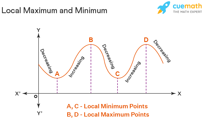
• Intervals of increase and decrease are:

  • sets of x values where the graph is increasing (+ slope) /

  • sets of x values where the graph is decreasing (- slope)\

• Local max is the point on a graph that is larger than all other values in its immediate vicinity.

• Local min is the point on a graph that is smaller than all other values in its immediate vicinity.

• The absolute max/min is the value of the graph that is largest or smallest over its entire domain.

  • ± infinity are not considered as absolute value points

    

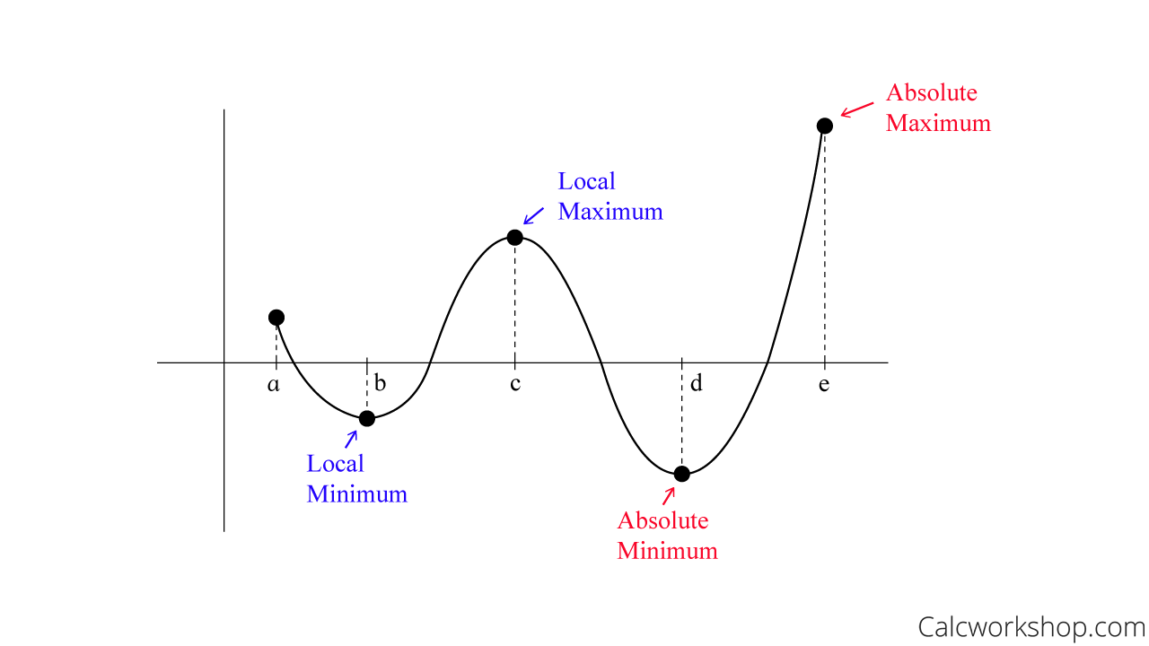
• Turning points are the absolute/local max/min points where the domain continues on either side.

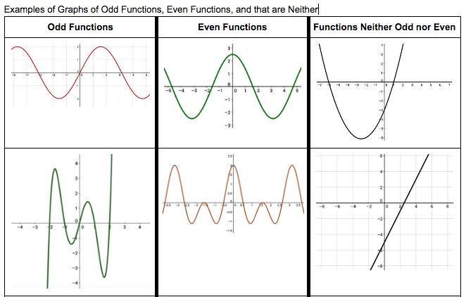
• Even functions are symmetrical on the y-axis

  • f(-x) = f(x)

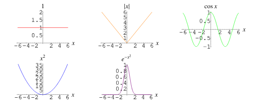
• Odd functions are symmetrical on the x-axis

  • f(-x) = -f(x)

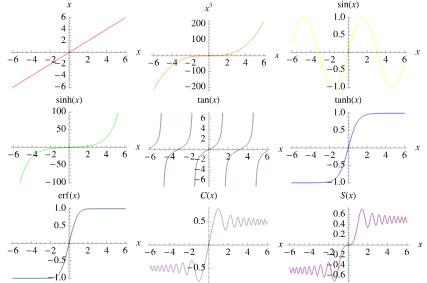
• Most functions are neither even or odd

• When combining functions by addition:

  • Zeroes exist when f&g are equal distances from the x-axis but opposite signs.

  • add y-coordinates

  • The domain of the combined function is the overlap of D_f and D_g

  • Any point where F & G intersect will be doubled in the new combined function

• When combining functions by subtraction:

  • Zeroes occur where f & g intersect

  • subtract y-coordinates

  • The domain of the combined function is the overlap of D_f and D_g.

• When combining functions by multiplication:

  • All the zeroes of both functions are zeroes in the new function

  • Multiply y-coordinates

  • if f & g are polynomials, the new function will have the sum of both degrees

  • The domain of the combined function is the overlap of D_f and D_g.

• When combining functions by division:

  • Zeroes are where the numerator has zeroes

  • vertical asymptote on the new function is where the denominator has zeroes

• When taking the reciprocal of a function:

  • Where the y values of the original function approach ± infinity, the reciprocal will approach 0

  • if the original function has 0, the reciprocal will turn these zeroes into vertical asymptotes

  • intervals of increase become intervals of decrease

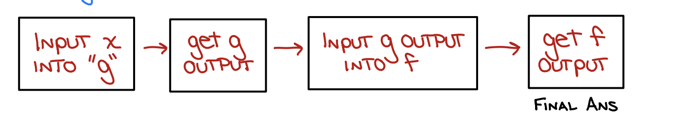
composition

• f _^o g means f composed with g

  • f(g(x))

Unit two - Polynomials

• The degree of a polynomial is the highest exponent of the variable

• The leading coefficient is the coefficient of the term with the highest power

  • 1^st degree → linear

  • 2^nd degree → quadratic

  • 3^rd degree → cubic

  • 4^th degree → quartic

• A linear factor means that a straight line passes through the zero

• A quadratic factor means that the curve has a turning point at zero

• A cubic factor means that the zero has a cubic squiggle

End behaviours

• when the degree is even,

  • (+) leading coefficient: as x→ ± infinity, y→ + infinity

  • (-) leading coefficient: as x→ ± infinity, y→ - infinity

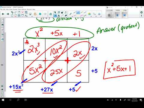
Dividing Polynomials:

• dividend = divisor x Quotient + remainder

• When dividing polynomials, use the chart method

  • put the 1st term in the upper left box, then use multiplication on the outside to complete.

• To figure out the perfect factors of a polynomial

  • factors of the constant (term with an x)/ factors of the leading coefficient

    • when plugged in the equation, it should equal to 0

    • When you have the factor, use it as the divisor to divide the polynomial

• Remainder theorem:

  • When a polynomial function is divided by (x-k), the remainder Is p(K)

  • When a polynomial function is divided by (jx-k), the remainder p(k/j)

• Factor theorem:

  • When a polynomial, p(x), has a factor (x-K), p(k)=0

  • When a polynomial, p(x), has a factor (jx-k) p(j/k)=0

Factoring

• Steps to factor polynomials:

  • Always common factor first

  • If it is a binomial, use the difference of square or sum/difference of cubes

  • If it is a trinomial, use a tricky trinomial chart or decomposition

  • if there are more than three terms, try factoring by grouping or factor theorem

• Steps to solving polynomial equations:

  • Rearrange the equation such that all terms are on the same side

  • Factor polynomials to determine the solutions

    • a polynomial has the same number of roots as the number of the degree of the polynomial but has less than or equal to the number of the degree

      • ex. a 4^th degree polynomial will have four roots, but may have two zeroes

    • Even degree polynomials can have no zeroes

    • Odd-degree polynomials must have at least one zero

Solving inequalities

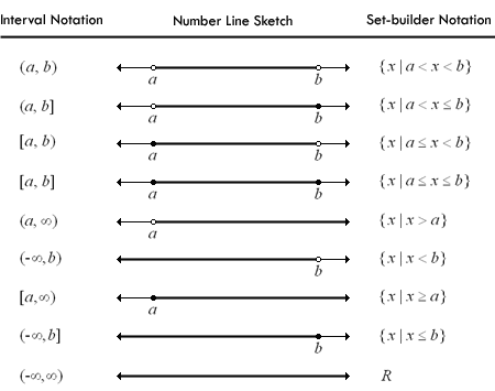
• ( : exclde that value

• [: include that value

  • ± infinity aren’t included in interval notation - use (_)

• To solve linear inequalities:

  • rearange so the variable is on one side of the equation and the constant on the other

  • when multiplying/dividing both sides by -1, the inequality sign flips

    • -x<3 → x>-3

  • When you have inequalities on both sides, solve them as two separate inequalities

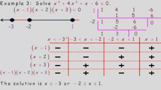
• To solve polynomial inequalities:

  • factor the expression and use its factor in a chart.

Unit three - Rationals

• A rational function is in the form of f(x)/g(x)

  • y-int is when x=0

  • the zeroes of the numerator are the zeroes of the function

  • the zeroes of the denominator are the vertical asymptotes of the function

  • Domain is all the real numbers except the zeroes of denominator

• If the degree of the numerator is smaller than the degree of the denominator, there is an horizontal asymptote at y=0

• If the degree of the numerator is equal to the degree of the denominator, the horizontal asymptote is the product of the leading coefficient of f(x)/ leading coefficient of g(x).

• If the degree of the numerator is one + the degree of the denominator, there is an oblique asymptote ( quotient of f(x) divided by g(x))

  • 

• To solve rational equations:

  • rearrange to make one side equal to 0

  • write as one rational expression

  • factor fully

  • state the roots

• Solving rational inequalities:

  • reagange and write one fully factored rational expression on one side with zero on the other side of the inequality

  • determine the zeroes and VAs

  • use a table to determine whether the function is positive or negative on each interval

Unit four - trigonometry

Trignonometry part 1:

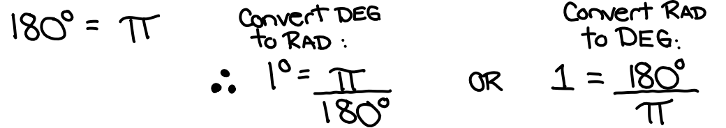
• Radians are another way to measure angels using the distance travelled around a circle’s circumference (no units)

  

  • π → 180º (half circle)

  • 2π → 360º ( full circle)

  • π/2 → 90º

  • 3π/2 → 270º

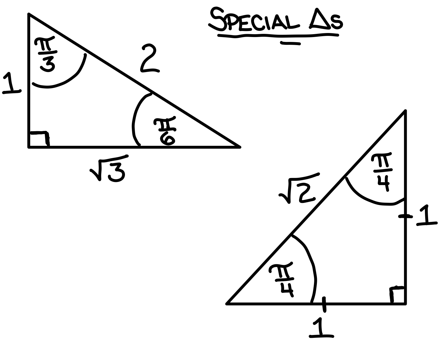
  • π/3 → 30º

  • π/4 → 45º

  • π/6 → 60º

• When transforming sinusoidal functions:

  • amplitude → Vertical stretch

  • axis → vertical translation

  • period → horizontal stretch

    • sin → 2π

    • cos → 2π

    • tan → π

      • to find period, 2π*k = period

        • or π*k = period for tan

  • phase shift → horizontal translation

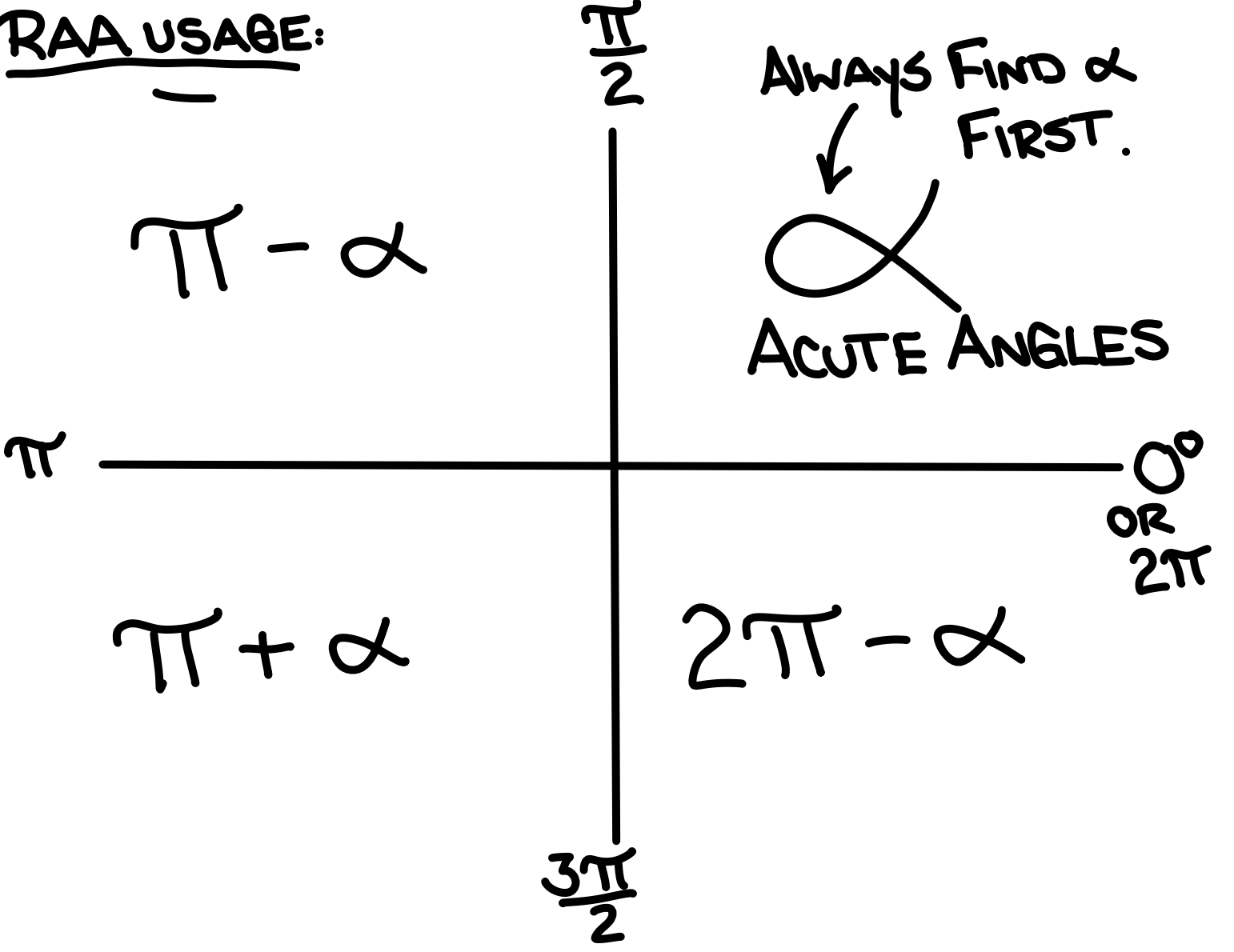
• If an angle is in standard position, the acute angle between the terminal arm and the horizontal axis is the RAA.

• the CRAA is the “compliment” of the RAA; the acute angle between the terminal arm and the y-axis

  

• Co-functions:

  • sin & cos

  • sec & csc

  • tan & cot

• Compound angle formulas:

  • cosine → cos(z+a) = cosz*cosa - sinz*sina

    • cos(z-a) = cosz*cosa + sinz*sina

  • Sine → sin(z+a) = cosz*sina + cosa*sinz

    • sin(z-a) = cosz*sina - cosa*sinz

  • Tangent → tan (z+b) = (tanz+tanb)/ (1-tanztanb)

    • tan (z-b) = (tanz-tanb)/ (1+tanztanb)

• Double angle formulas:

  • cosine → cos²a -sin²a

    • 1-2sin²a

    • 2cos²a -1

  • sine → 2(sina*cosa)

  • tangent → 2tana/(1-tan²a)

• Trig identities:

  • tan = sin/cos

  • sin² + cos² =1

  • cot = cos/sin

  • cos² = 1-sin²

  • 1+cot² = csc²

  • tan² +1 = sec²

  • 1/sin = csc

  • 1/cos =sec

  • 1/tan = cot

Trigonometry part 2:

• without a restricted domain, there are infinite repeating solutions

• To solve quadratic trig equations, change the trig ratio to a variable (x).

Unit five - Logarithms

• logarithms are the inverse of exponential functions

  • x=2^y → log₂x=y

• Properties of logarithms:

  • log_a1 =0

  • log_ab^x=x

  • a^logax=x

• Change of base formula:

  • log_ax =(logx)/(loga)

    • leave the answer in fractions, not decimals

• Laws of logarithms:

  • product law → log (m*n) = logm + logn

  • quotient law → log (m/n) = logm - long

  • power law → logm^a = a*logm

• All vertical work for exponential transformations becomes horizontal in logs