Chapter 12: Linear Regression and Correlation
Introductory
- Bivariate data: two variable data
- Multivariate data: more than two variables
12.1 Linear Equations
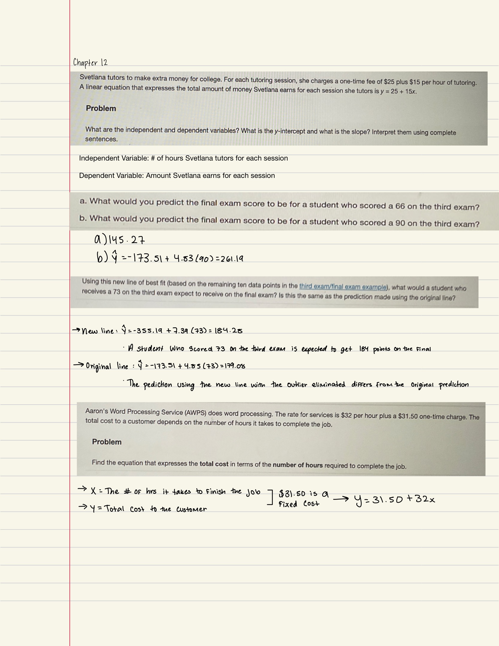
- y = a + bx: linear regression for two variables is based on a linear equation with one independent variable.
- Independent variable: x
- Dependent variable: y
- Slope: b
- y-intercept: a
- Graph form: a straight line or linear
- B > 0: slopes to the right
- b = 0: horizontal line
- b < 0: slopes downward to the right
12.2 Scatter Plots
- Scatterplot: uses dots to represent values for two different numeric variables.
- Calculator steps for scatter plot
- Enter your X data into list L1 and your Y data into list L2.
- Press 2nd STATPLOT ENTER to use Plot 1. On the input screen for PLOT 1, highlight On and press ENTER. (Make sure the other plots are OFF.)
- For TYPE: highlight the first icon, the scatter plot, and press ENTER.
- For X List, enter L1 ENTER and for Ylist: L2 ENTER.
- For Mark: it does not matter which symbol you highlight, but the square is the easiest to see. Press ENTER.
- Make sure there are no other equations that could be plotted. Press Y = and clear any equations out.
- Press the ZOOM key and then the number 9 (for menu item "ZoomStat"); the calculator will fit the window to the data. You can press WINDOW to see the scaling of the axes.
- Scatterplot Direction: High values of one variable occurring with high values of the other variable or low values of one variable occurring with low values of the other variable
- Strength: Looking at how close the points are to the line
- Linear regression: shows the relationship between a dependent and independent variable(s)
12.3 The Regression Equation
- Least-Squares Line: You have a set of data whose scatter plot appears to "fit" a straight line
- Least-squares regression line: Helps obtain a line of best fit
- y hat: estimates value of y
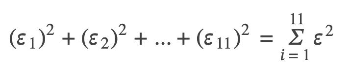
- y0 – ŷ0 = ε0: error or residual
- Absolute value of a residual: measures the vertical distance between the actual value of y and the estimated value of y
- ε: the Greek letter epsilon
- Slope equation: b = r (sy / sx)
- sx = the standard deviation of the x values.
- sy = the standard deviation of the y values
- Interpretation of the Slope: “The slope of the best-fit line tells us how the dependent variable (y) changes for every one unit increase in the independent (x) variable, on average.”
- Using the Linear Regression T Test
- In the STAT list editor, enter the X data in list L1 and the Y data in list L2, paired so that the corresponding (x,y) values are next to each other in the lists.
- On the STAT TESTS menu, scroll down with the cursor to select the LinRegTTest.
- On the LinRegTTest input screen enter: Xlist: L1 ; Ylist: L2 ; Freq: 1
- On the next line, at the prompt β or ρ, highlight "≠ 0" and press ENTER
- Leave the line for "RegEq:" blank
- Highlight Calculate and press ENTER.
- Correlation coefficient (r): is numerical and provides a measure of strength and direction of the linear association between the independent variable x and the dependent variable y.
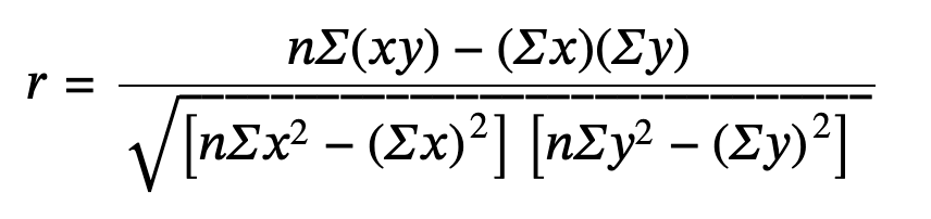
- The value of r is always between –1 and +1: –1 ≤ r ≤ 1.
- The size of the correlation r indicates the strength of the linear relationship between x and y. Values of r close to –1 or to +1 indicate a stronger linear relationship between x and y.
- If r = 0 there is likely no linear correlation. It is important to view the scatterplot, however, because data that exhibit a curved or horizontal pattern may have a correlation of 0.
- If r = 1, there is perfect positive correlation. If r = –1, there is perfect negative correlation. In both these cases, all of the original data points lie on a straight line.
- Positive correlation: A positive value of r means that when x increases, y tends to increase and when x decreases, y tends to decrease.
- Positive correlation: A negative value of r means that when x increases, y tends to decrease and when x decreases, y tends to increase
- Correlation does not imply causation
- 0 < r < 1: A scatter plot showing data with a positive correlation.
- –1 < r < 0: A scatter plot showing data with a negative correlation.
- r = 0: A scatter plot showing data with zero correlation.
- Coefficient of determination: a number between 0 and 1 that measures how well a statistical model predicts an outcome
- r^2 interpretation: when expressed as a percent, represents the percent of variation in the dependent (predicted) variable y that can be explained by variation in the independent (explanatory) variable x using the regression (best-fit) line.
- 1 - r^2 Interpretation: when expressed as a percentage, represents the percent of the variation in y that is NOT explained by variation in x using the regression line.
12.4 Testing the Significance of the Correlation Coefficient
- Significance of the correlation coefficient: to decide whether the linear relationship in the sample data is strong enough to use to model the relationship in the population.
- ρ: population correlation coefficient
- r: sample correlation coefficient
- Conclusion for Significant: There is sufficient evidence to conclude that there is a significant linear relationship between x and y because the correlation coefficient is significantly different from zero.
- Conclusion for Not Significant: There is insufficient evidence to conclude that there is a significant linear relationship between x and y because the correlation coefficient is not significantly different from zero.
- Null Hypothesis: H0→ ρ = 0
- Alternative Hypothesis: Ha→ ρ ≠ 0
- Interpreting Null Hypothesis: The population correlation coefficient IS NOT significantly different from zero. There IS NOT a significant linear relationship (correlation) between x and y in the population.
- Interpreting Alternate Hypothesis: The population correlation coefficient IS significantly DIFFERENT FROM zero. There IS A SIGNIFICANT LINEAR RELATIONSHIP (correlation) between x and y in the population.
- To calculate the p-value using LinRegTTEST
- On the LinRegTTEST input screen, on the line prompt for β or ρ, highlight "≠ 0"
- The output screen shows the p-value on the line that reads "p ="
- p-value is less than the significance level: We reject the null hypothesis. There is sufficient evidence to conclude that there is a significant linear relationship between x and y because the correlation coefficient is significantly different from zero
- p**-value is NOT less than the significance level**: DO NOT REJECT the null hypothesis. There is insufficient evidence to conclude that there is a significant linear relationship between x and y because the correlation coefficient is NOT significantly different from zero.
12.6 Outliers
- Outliers: are observed data points that are far from the least squares line.
- Influential points: observed data points that are far from the other observed data points in the horizontal direction. These points may have a big effect on the slope of the regression line.
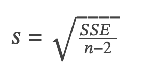
- Degrees of freedom: n - 2
Examples