W3: Advanced MRI modalities

Topic 1: Physiological & physical basis of functional Magnetic Resonance Imaging

Review of neurons & basic neural activity

Neurons = fundamental of unit of the CNS

• Propagate information via 2 processes:

  1. Transmission of altered electrical potential

  2. Release of neurotransmitters

The generation of spontaneous electrical activity by neurons is known as action potentials.

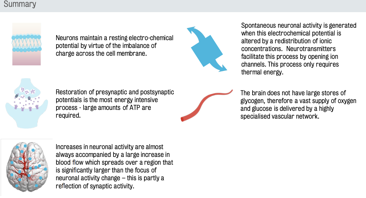
• Neuronal membrane is a lipid bi-layer which ① serves as an insulator & ② controls the diffusion of ions across the membrane

⚠ Ionic concentrations across the membrane are 🚫 balanced, i.e. they’re different on either side of the membrane

• K⁺ ions s have a higher concentration in the intracellular space

• Na⁺ & Cl^- ions have a higher concentration in the extracellular space

• :. neurons do not exist at a neutral electrical potential (finite electrical potential)

  • Membrane potential sits between -80mV and -40mV

Neurons are able to generate spontaneous electrical activity by transporting ions across the neuron membrane.

• Achieved by moving ions through ion channels.

• Two types of ion channels: ion channels vs ion pumps (require additional energy)

Transmission of an electrical potential requires kinetic energy only; however, repolarisation of the membrane (i.e., restoration of ionic concentration to pre-neuronal activity levels) requires an input of energy to the tissue.

• Additional requirement for energy can only be met by increases in tissue metabolism

2^nd mechanism allowing for the transport of information via neurons: neurotransmitters

• Have endogenous chemicals that transmit signals across the synapse by opening ionic channels

• Are packed into synaptic vesicles in the presynaptic side & bind to specific receptors in the postsynaptic side

• Are classified according to their molecular character

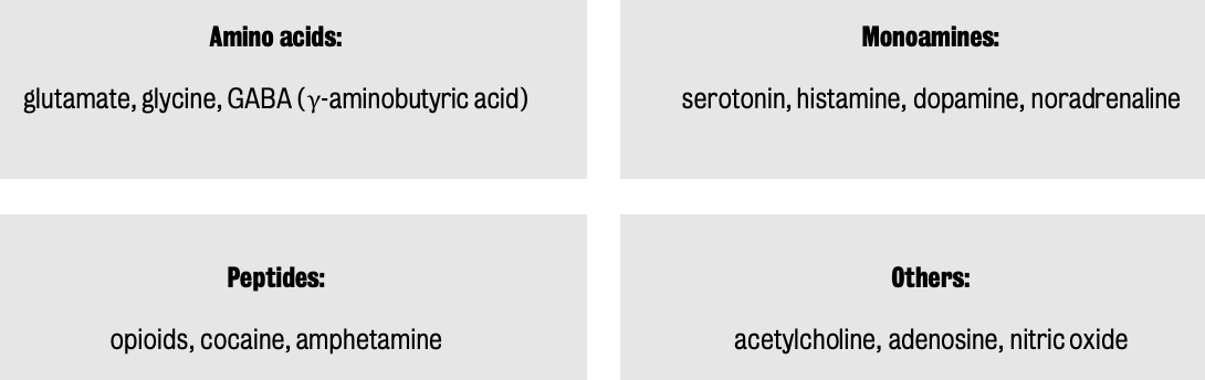
Neurotransmitter re-uptake in pre-synaptic space is essential to maintain neuronal activity.

• Concentrations of neurotransmitters must be restored to their original levels in the presynaptic side in order for neurotransmitter activity to continue

• Reuptake and recycling also requires additional energy

Adenosine triphosphate (ATP) = energy currency of the brain

• Manufactured from fatty acids, ketone bodies and glucose

• Concentration of ATP in the brain is relatively constant :. precursor molecule glycogen has low concentrations

Breaking down of glycogen (glycosis)

• Glycogen produces (→) pyruvate → ATP

• Glycosis processes: aerobic or anaerobic

The human brain cannot properly function with considerable concentrations of lactate :. the aerobic pathway is preferred.

Synaptic density in the human brain is very large & energy requirements in synapses are mainly met by oxidative glycolysis.

The brain requires real-time replenishment of energy in order to support its metabolic processes :. it needs to obtain oxygen and glucose from the arterial blood supply.

• Brain consumes 20% of all arterial blood :. 20% of all the oxygen generated by the heart and lungs.

  • :. Functional neuroimaging techniques, which are sensitive to correlates of blood flow or metabolism, can be used to make inferences about brain activity.

Arterial network

• Deals with brain’s huge energy demands

What happens after arterial oxygenated blood leaves the heart?

1. Vessel diameter of the artery is reduced

   • Thinning of capillary network → large density of capillary distribution throughout the human brain, allowing for very close proximity to the cells & very efficient transport of oxygen and glucose.

2. Arterial blood velocity changes

   • Facilitates the transport of oxygen and glucose to the neurons by slowing down arterial blood flow.

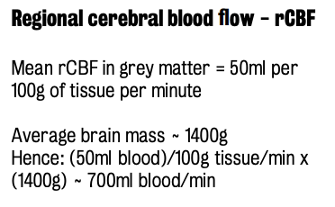
   • Regional cerebral blood flow (rCBF) = amount of blood flowing to specific regions of the brain within a given time

PET and fMRI rely on the consistent relationship between regional changes in neuronal activity in the brain & changes in microcirculation (i.e.,g rCBF metabolism and oxygenation)

⭐ ️Neurovascular coupling involves the mechanisms by which increases in the activity of neurons trigger the production of substances that relax the smooth muscle wall of arteriole in order to increase their diameter and deliver an increased amount of blood

• Responsible molecule = nitric oxide, which can be secreted by astrocytes after changes in neural activity

Understanding the basic principles of BOLD fMRI

Increase in cellular activity → increase in blood flow

In red blood cells, oxygen is transported by haemoglobin.

• Haemoglobin = protein complex with four structures known as heme groups, each of which carry oxygen

Magnetic properties of haemoglobin

• Oxygenated haemoglobin: diamagnetic

• Deoxygenated haemoglobin: paramagnetic, meaning it can acquire magnetic properties in the presence of an external magnetic field

  • The 4 unpaired electrons abandoned when haemoglobin gives up its oxygen are responsible for giving oxygenated haemoglobin its’ strong paramagnetic.

Magnetic susceptibility = physical parameter that describes the magnetic character of a molecule (or substance).

• Deoxygenated haemoglobin has larger magnetic susceptibility due to its 4 unpaired electrons

• Presence of molecules with different magnetic susceptibility → ability to distort the uniformity of the magnetic field

  • MR signal in the vicinity of regions with large magnetic susceptibility will decay more rapidly due to distortion of the magnetic field.

Thulborn et al. (1982)

• Transverse relaxation rate governs amplitude of the signal present in our image

  • Transverse relaxation rate of the MR signal is hugely dependent on the oxygenation state of blood :. it decays significantly faster in the presence of deoxygenated blood.

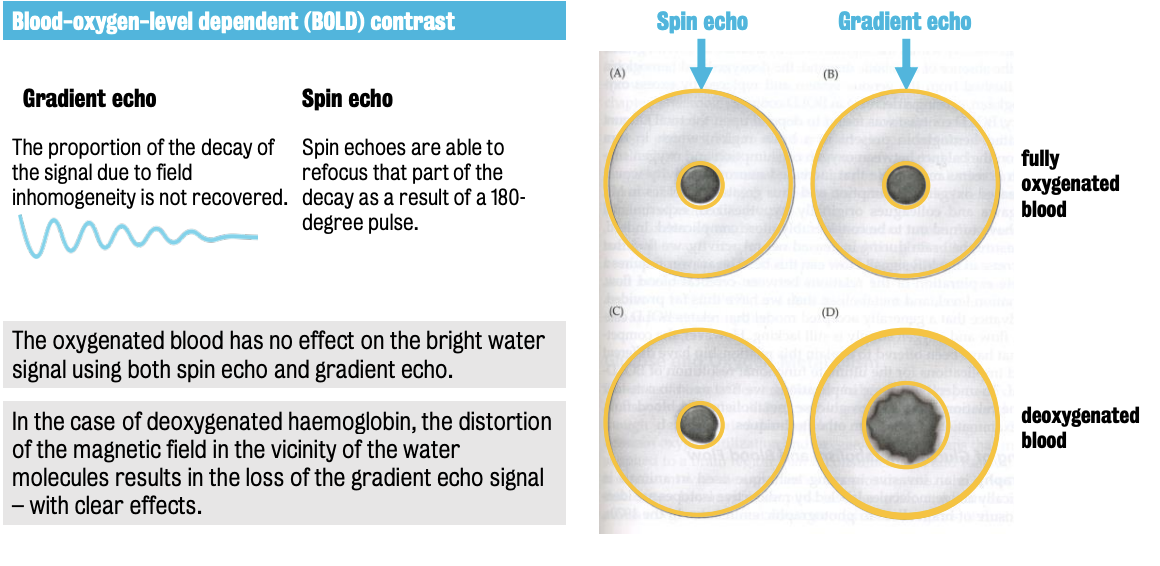
Seiji Ogawa (1990) — Demonstration of blood oxygenation’s effect on MR images using grading echoes and spin echoes images

• Gradient echos are formed by the reversal of magnetic field gradient

• Oxygenated blood has no effect on the water signal

• Coining of ‘BOLD’ term emerged as a result of this experiment

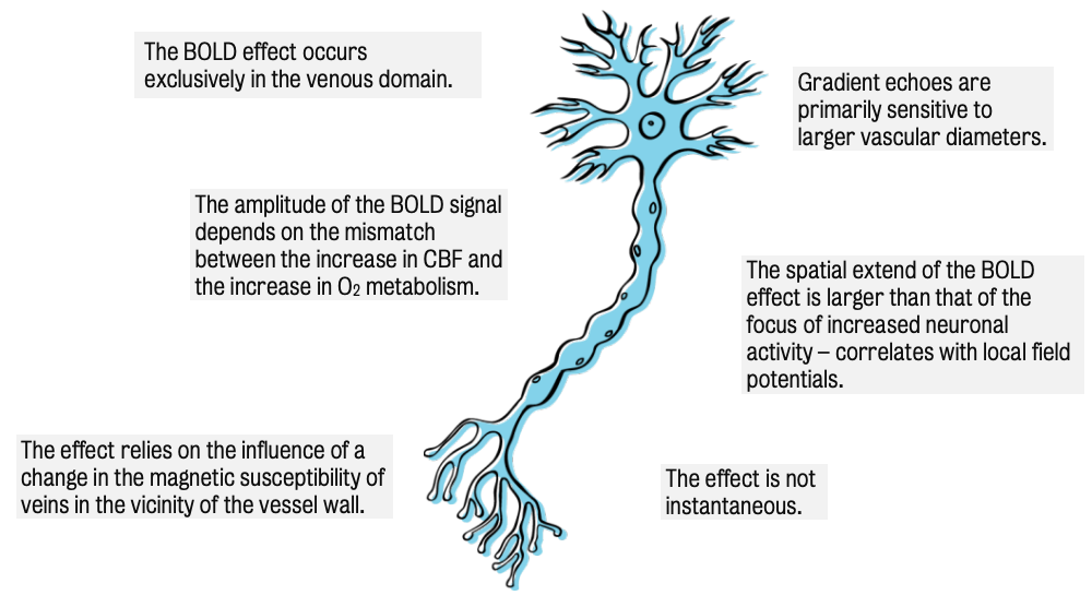
Amplitude of the BOLD contrast depends on oxygen metabolism

• BOLD construct depends on the relationship between the oxygenation content of the tissue which is governed by rCBF & cerebral metabolic rate of oxygen consumption.

• Bold contrast directly proportional to depth of anaesthesia in rodent

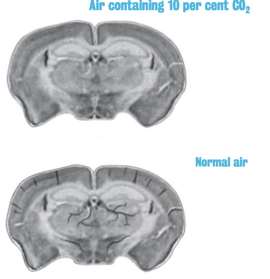
Caption: (top) dark vein effect disappear due to diamagnetic properties of oxygenated haemoglobin; (bottom): deoxygenated haemoglobin distorts magnetic fields, :. veins appear dark

Reactive hyperaemia

• Refers to phenomenon by which blood flows to an area following a period of reduced blood flow

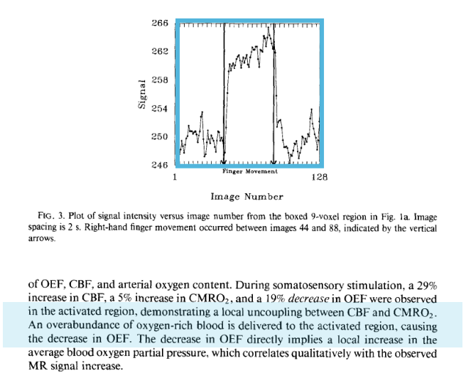
• Low changes in the rate of consumption of oxygen by the neurons despite large increase of oxygen being delivered to the neurons

  • Suggesting that oxygen extraction fraction actually decreased during activation

Bandettini et al. (1992) — BOLD contrast in obtaining fMRI images

• Reactive hyperaemia → measurable increase in the amplitude of the signal

• Overabundance of oxygen-rich blood delivered to the active region, causing a decrease in the oxygen extraction fraction (OEF)

Recap:

Increase in the local rate of utilisation of oxygen (in given brain region) → Increase in feed-back concentration of deoxygenated haemoglobin → CBF increase (due to neurovascular coupling & reactive hyperaemia) → overabundance of oxygenated haemoglobin (delivered to that brain region)

Unused oxygenated haemoglobin molecules will go back into venous return :. relative concentration of deoxygenated haemoglobin will reduce

Rise in the use of BOLD fMRI since its inception in 1992

• Application in task-activated paradigms & studies of resting state functional activity & event-related designs

• Non-invasive

• Sensitive to modulation by psychotropic drugs (:. huge application in pharmacological imaging)

BOLD signal is primarily related to synaptic and post synaptic activity.

• BOLD signal does not have a close relationship with the electrical activity of neurons

  • Why? BOLD signal depends on the supply of oxygen to the neurons to maintain this activity, meaning it is primarily related to synaptic and postsynaptic activity

There is no conclusive answer as to why reactive hyperaemia occurs.

Topic 2: Introduction to diffusion imaging & Tractography

Basic principles of diffusion imaging and tractography

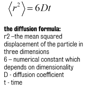
Diffusion = simple random movement of water molecules

• Mean square displacement increases over time

• Diffusion coefficient is directly related to mobility of water molecules and kinetic energy (& :. temperature)

  • Due to the ~ constant temperature of the human body, the diffusion coefficient of water is also constant in the human body/brain

⚠️ Presence of different biological structure (other than water) might affect the mobility of water molecules in the brain.

• All cells, membranes & fibres act as obstacle for water molecules and reduce their displacement.

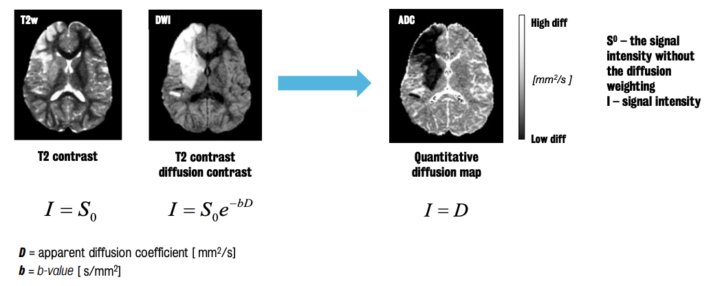
Apparent diffusion coefficient (ADC) describes the mobility of the water molecules inside biological tissues

• Key point of diffusion imaging: Understanding underlying microstructural organisation of biological tissue by measuring the displacement of water molecule in a fixed amount of time.

Diffusion MRI is a non-invasive, in-vivo technique that allows for the measurement of molecular diffusivity of water inside biological tissues

• Displacement is very small b/c the time allocated to molecule diffusion is short (~20-40 millisecond)

• Water molecules probe tissue structure at a microscopic scale → high imaging resolution thanks to a high sensitivity to detect light & early changes in cellularity or structure organisation

Measuring diffusion:

MR scanner collects 2 types of images: T2-weighted image & a diffusion weighted image

• Difference: ⭐️ DWI is T2 weighted with the added diffusion contrast

• b-value is not unique. It’s the amount of diffusion contrast we want to add in our diffusion image (:. can change according to diffusion experiment)

  • Higher the b-value → stronger diffusion contrast & signal attenuation

  • Normal b-value for standard DTI analysis is b 1000

Diffusion is a 3D process, :. by probing diffusion along different directions, we may encounter different results.

• Isotropy (isotopic diffusion) refers to tissue with the same diffusion property along every direction.

  • Said of homogenous tissue where water molecules are free to diffuse along every direction equally

• Anisotropy (anisotropic diffusion) refers to tissue with a different diffusion properties along different direction

  • Said of heterogeneous tissue with very strong structural organisation

  • Presence of fibres here hinders the mobility of water molecules perpendicular to the direction of the fibres but not along them

  • Axons and white matter are the main regions where anisotropy is observed (b/c axonal membranes & myelin sheets restrict diffusion across fibre)

Early interpretations of diffusion imaging maps were challenging due to heavily head orientation & diffusion direction dependent nature of these maps, making anisotropy resemble lesions.

Diffusion tensor imaging (DTI)

DTI was introduced in 1994 by Petter J. Basser

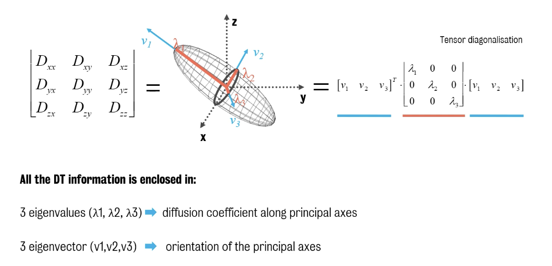
Diffusion tension = mathematical formula that creates a 3D model of water molecular diffusion inside each voxel of the brain

• Obtained by measuring the diffusion along multiple direction

  • Minimum = 6 (number of parameters needed); better estimate ~ 20 parameters

• Allows us to extract for each voxel of the brain a 3D model of water diffusivity

Diffusion ellipsoid represents the actual 3D displacement water molecules in a fixed amount of time & captures all the information available in the diffusion tensor

• NOT a simplification

Tensor diagonalisation → 3 eigenvalues

• Eigenvalues represent the diffusion coefficient along the three principal axes on the left side

  • Vectors that tell us the orientation of these principal axes of the ellipsoid :. how the ellipsoid or the diffusion tensor is oriented in space

• Size & shape are fully defined only by the three eigenvalues,

Measures extractable from DTI

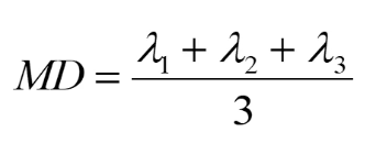
1. Mean diffusivity (MD)

   • Identifies average mobility/diffusivity of water molecule (average ADC value) irrespective of direction

   • Rotation invariant index: doesn’t change with the orientation of the subject in the scanner

   • Can detect small changes in the brain

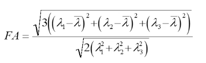
2. Fractional anisotropy (FA)

   • Informs the organisation of the brain microstructure

   • Changes in FA can be used to detect biological changes

   • Rotational invariant index

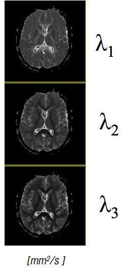
Eigenvalue maps

• ƛ1 (lambda 1) = largest eigenvalue & represents diffusion along the direction of maximum diffusivity (or ‘axial diffusivity)

  • Similar to longitudinal diffusivity map ADC //

• ƛ2, ƛ3 or ADC_┴ maps show the perpendicular diffusivity of fibres

  • Similar to transverse diffusivity map ADC_┴ = (ƛ2 + ƛ3)/2

The list of all DTI applications is quite lengthly as DTI is applied practically everywhere.

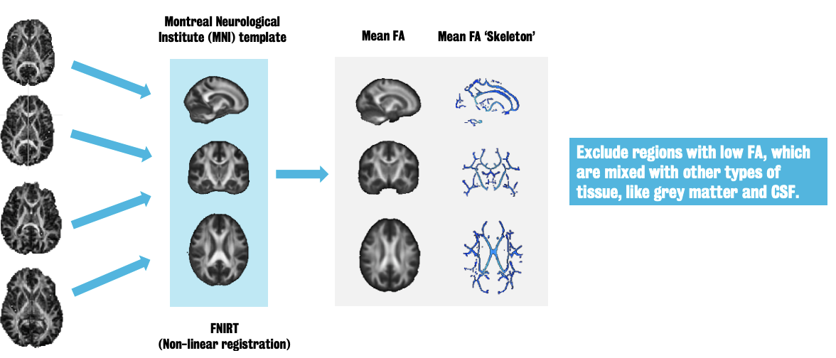
Tract-based spatial statistics (TBSS)

• Common approach to using and analyzing DTI maps focused on normalizing all maps to a standard template (i.e., MNI or the Montreal Neurological Institute template) to calculate the mean FA for all subjects and extract a skeleton, representing only the core of all white matter region

• 2^nd registration step: refining subject registration by better aligning only the white matter region of interest.

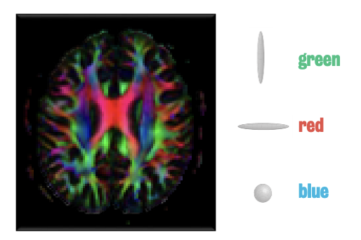
Main use of the direction information of each tensor: to connect together different voxels according to their underlying white matter orientation (diffusion tractography)

• By assigning colour FA map, we can get a distinct colour for each voxel based on the tensor orientation

  • RBG map or colour maps are useful to check that colours are correct and therefore diffusion orientation are correctly aligned

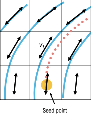
Diffusion tractography (or fibre tracking)

Each main eigenvector is tangential to the underlying white matter

• Streamline tractography: starting from a seed voxel (or point), we can start to propagate a 3D curve representing the white matter track

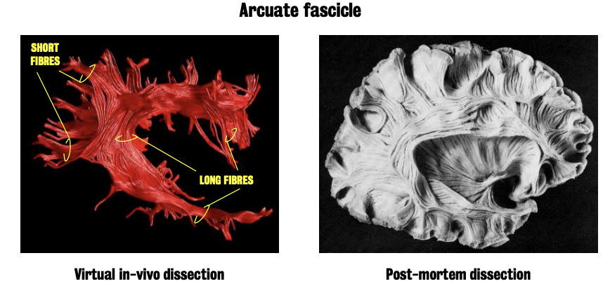
Tractography is simply a mathematical approximation based on the underlying movement of water molecules :. while post-mortem sample may allow for ample white matter visualisation, it may not be perfectly accurate

In DTI tractography, there are two main criteria to track and stop tracking:

1. Anisotropy threshold

   • Used to limit tracking only within white matter regions

   • Start if FA > threshold and stop if FA < threshold (FA ~0.15/0.20)

2. Angle threshold

   • Used to limit the angle between two subsequent steps of the tractography algorithm

   • Stop if the angle between the old and new direction is > threshold

Tractography allows us to use tracts as 3D regions to extract quantitative measure

• Can be adapted to anatomy of each individual subject :. is more sensitive to changes in white matter

Methods of extracting measures:

1. Sample measurements

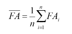
   • Sample FA at each step and calculate mean of all samples

2. Along-tract measurements

   • Looks at local changes along track measure that might not be visible in the whole average of the track.

     • e.g., dispersion, crossing, bending

⚠ Tractography can generate spurious streamlines, showing invalid or missing connection

Potential issues with tractography

• Data quality

  • Noisy data set can introduce spurious artefacts

  • High-quality resolution is key

• Diffusion model limitations

  • Cannot resolve multiple fibre orientation or fibre crossing

• False negative

  • Occurs because we expect to see fibres that are not reconstructed

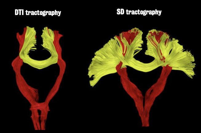
A new method called spherical deconvolution (SD) is able to resolve crossing issues

• For each voxel, we can see multiple lobes, each representing an actual fibre orientation

  • This allows us to reconcile expected callosal anatomy

• Allows us to map tracts that could not be visualized with normal diffusion tensor imaging

Topic 3: Magnetic Resonance Spectroscopy (MRS) of the brain

NMR = nuclear magnetic resonance spectroscopy

MRS = magnetic resonance spectroscopy

MRI = magnetic resonance imaging

These techniques all rely on magnetic resonance (MR) phenomena

Today, NMR refers to chemical analysis

• Used for structural elucidation of compounds, macromolecules & metabolomics

• Unlike MRS and MRI where subjects are inserted horizontally into the magnet, NMR samples are put in glass tubes and performed on instruments with an upright magnet where the sample is introduced from the top

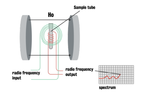
NMR and MRS data comes in the form of a trace or spectrum.

MRS and MRI are based on the same magnetic resonance phenomena, but are conducted in different ways:

• MRS focuses on the metabolites in a volume (or voxel) using localization techniques

  • Detects metabolites present in millimolar concentrations.

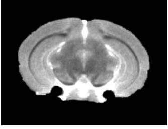
• MRI look at water protons whose magnetic properties change depending on its environment

  • T1 and T2 values can be affected by the local microstructure or ion concentrations

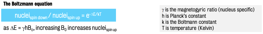
💬 Spin-up protons have relatively lower energy than the spin-down protons

:. It’s excess of spin-up protons give rise to the MR signal

Protons give rise to peaks at different positions on the chemical shift scale, i.e., they resonate at different frequencies (due to the presence of chemically bonded electrons).

• Difference in resonance frequencies give rise to the chemical shift.

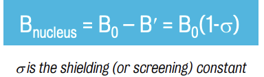
• Electrons are moving particles, i.e. charged :. induce a magnetic field B’, opposed to the main magnetic field B₀

This means that protons experience a magnetic field that is lesser than the applied magnetic field, i.e., it is shielded from the magnetic field.

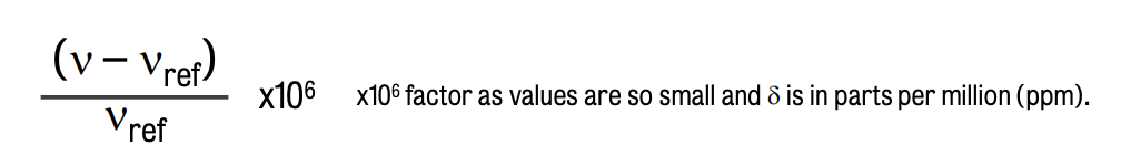
Chemical shift (i.e., 𝛿 delta) indicates the location of the peak on the spectrum

• Chemical shift value of a peak is given by the frequency difference between a signal and a reference signal

TSP (sodium d₄-trimesthylsilylpropionate) is commonly used as a standard in NMR

• Both a chemical shift reference & a concentration reference

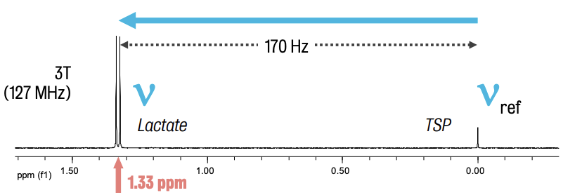
Caption: Difference in the resonance frequency of the TSP protons and the methyl protons of lactate = 170 hertz.

By using the chemical shift scale, we can compare spectra measured at different field strengths.

• ⚠ We cannot put in a reference compound in MRS, so we use an internal reference (usually water or creatine)

Ethanol NMR spectrum

Oxygen is much more electronegative than carbon, :. will pull bonding electrons to itself from the adjacent bonded proton. As a consequence, hydrogen attached to oxygen is less shielded than from the applied magnetic field, and resonates at lower frequency than the protons attached to carbon.

Peaks (resonances) have chemical shift value, but may also undergo spin-spin coupling → splitting of the single resonance to a multiple resonance

Spin-spin coupling (aka scalar coupling or J-coupling) arises from interactions between adjacent bonded magnetic nuclei

• Measured in Hz & is field-independent

• Through-bond effect: nuclei only couple with other nuclei that they're bonded to & strength of the coupling decreases with the increasing number of bonds between them

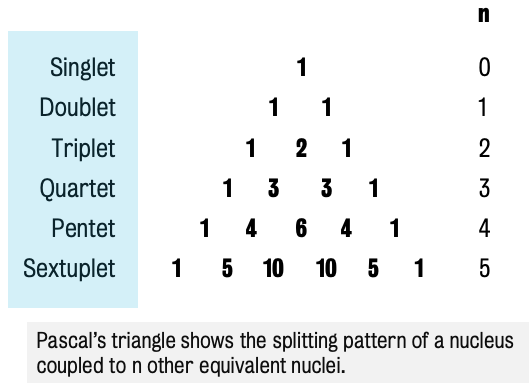
  • Reason behind why lactate methyl protons give rise to a doublet

Pascal’s triangle identifies how many split peaks there are and the ratio of the split peaks according to how many nuclei a nucleus is coupled with

In spectroscopy, there is a greater dispersion of resonances as we go to high field strengths, meaning we can resolve them better as they're not so overlapped.

Part 2:

Quantification of Metabolite Concentrations: MRS allows for the estimation of metabolite concentrations in specific brain regions.

• The area under each spectral peak is proportional to the number of protons of a specific metabolite, assuming complete T1 relaxation.

• Absolute quantification is challenging in vivo, often requiring a reference standard like water or normalization to the creatine signal.

  • Challenges of In Vivo MRS: Spectra obtained from living brains are less refined than those from high-resolution spectrometers on small samples.

• In vivo spectra exhibit broader peaks due to magnetic field inhomogeneities, making the quantification of numerous chemicals more difficult compared to in vitro samples.

Software for Spectral Analysis: LCModel is a commonly used software package for quantifying metabolite concentrations.

• LCModel works by fitting model spectra (experimentally acquired or computationally simulated) to the acquired in vivo spectrum.

Technical Considerations in MRS Acquisition: Several techniques are employed to enhance the quality of MRS data.

• Water and Lipid Suppression: The high concentration of water and lipids can obscure metabolite signals, necessitating suppression techniques and careful voxel placement.

• Voxel Selection: Similar to MRI, slice-selective RF pulses combined with magnetic field gradients are used to define the volume of interest (voxel) from which the signal is acquired. Saturation pulses can further refine voxel edges.

• Chemical Shift Displacement: Due to the relationship between frequency and position in the presence of a gradient, spectral lines from different chemical shifts originate from slightly different voxel locations, introducing a potential error.

• Echo Time (TE) Dependence: MRS spectra can be acquired with short or long echo times, each offering different advantages and disadvantages.

• Short TE: Higher signal-to-noise ratio and allows detection of short T2 species like myo-inositol, but suffers from a complicated baseline due to macromolecules and lipids.

• Long TE: Simpler baseline, but quantification is complicated by the need to account for T2 relaxation.

Key Brain Metabolites Detectable using Proton MRS: The lecture describes several important metabolites and their significance:

• N-acetyl aspartate (NAA): Predominant peak, marker of neuronal and axonal integrity. Levels can decrease in neuronal loss and increase in Canavan's disease.

• Creatine (Cr): Involved in energy metabolism, relatively stable, often used as an internal standard. Levels can decrease in cell death and increase after head trauma.

  • Creatine is the sum of free creatine and phosphocreatine

• Choline (Cho): Peak reflects soluble membrane phospholipids and is associated with membrane turnover, myelination, and inflammation. Often suggested to reflect overall cell density.

• Myo-inositol (MI): Thought to be involved in osmotic regulation, often considered an astrocyte or glial cell marker, best seen at short TE. Increased in some dementias and HIV infection.

• Glutamate (Glu) and Glutamine (Gln): Major excitatory neurotransmitter and its precursor. Often measured together as Glx at lower field strengths. MRS detects metabolic glutamate and the neurotransmitter pool.

  Glutamate is one of the most abundant compounds detected with protein MRS, and is released by approximately 90 per cent of excitatory neurons. MRS detects metabolic glutamate, as well as the neurotransmitter pool, and it's been suggested that glutamine levels may be a better measure of glutamate/glutamine cycling.

• GABA: Inhibitory neurotransmitter, difficult to quantify with standard MRS due to low concentration and J-coupling, requiring specialized pulse sequences like MEGA-PRESS. Because of this, it's difficult to quantify in standard MRS and requires specialized pulse sequences, such as MEGA-PRESS. As for glutamate, MRS 'sees' the total amount of GABA.

⭐️ Glutamate and glutamine have overlapping peaks at the low field, so sum of glutamate and glutamine is measured. GABA peaks overlaps peaks from glutamate and glutamine.

• Lactate: Not typically seen in the normal brain, its presence suggests anaerobic metabolism. Characterized by an inverted doublet at intermediate TE. Increased in hypoxia, ischemia, and some tumours.

  • Not typically seen in the normal brain, and its presence usually signifies interruption of oxidative phosphorylation and the start of anaerobic glycolysis.

  • Increased lactate is seen in hypoxia and ischemia.

• Lipids: Not normally visible in the brain; their presence may indicate tumours or contamination from scalp fat.

  • Range: 0.9 to 1.5 ppm

Spectra are similar across species (e.g., mice and humans), facilitating the translation of basic research findings to clinical applications.

Changes in the concentrations of specific metabolites are associated with various neurological and psychiatric conditions.

Key Takeaways:

• MRS is a valuable neuroimaging technique that provides insights into the brain's neurochemistry in vivo.

• Quantification of absolute metabolite concentrations is technically challenging, and relative measures are often used.

• Careful consideration of acquisition parameters (e.g., TE, voxel placement) and potential artifacts (e.g., lipid contamination, chemical shift displacement) is crucial for accurate MRS studies.

• Different echo times allow for the optimal detection of different metabolites.

• The concentrations of key brain metabolites like NAA, creatine, choline, myo-inositol, glutamate/glutamine, GABA, and lactate can provide valuable information about neuronal health, energy metabolism, membrane integrity, and neurotransmitter systems.

• MRS has significant potential for investigating the neurochemical underpinnings of neurological and psychiatric disorders and for translating preclinical findings to clinical settings.

Topic 4: Functional MRI data analysis

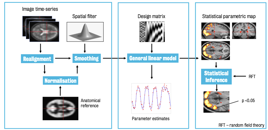
A typical fMRI analysis involves:

1. Preparing data for analysis

2. Building a model & fitting it to the data to determine the degree to which predictors explain the observed fMRI signal

3. Determine statistical significance

Primary role of preprocessing is to prepare data for subsequent analysis.

• Brains differ subtly in terms of size, shape and how they're crammed into the skull, making it more difficult to draw inference about the brain activation

  💡 There is also a need to correct for individual differences in how people move in the scanner.

Key concepts in fMRI preprocessing:

⚠ There is no single, perfect pipeline that will suit every data set. Each analysis requires trade-offs between correcting errors in the data and introducing new ones.

Universally agreed upon preprocessing steps:

• Motion correction

• Normalisation to standard space

• Image smoothing (or blurring)

Salient features of preprocessed images include:

• Resolution

• Signal-to-noise ratio

• Contrast between tissue types

• Distortions or signal loss

Significant difference between images represent a challenge to processing

Transformation is the 1st key concept of preprocessing

• Translations along the x, y & z axes

• Rotations around the x, y & z axes

• These 6 degrees of freedom are termed “rigid body registration’

Affine registrations uses zooms on the x,y and z axes, permitting 12 degrees of freedom

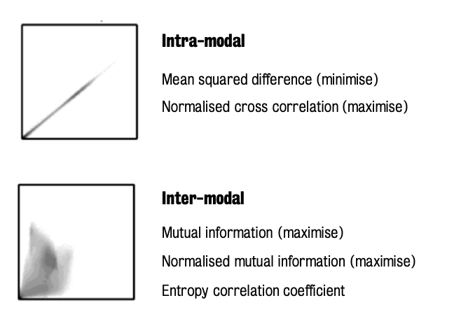
Objective or cost functions are measures of how well-aligned two images are

• Typically used when aligning images that do not look very similar, such as aligning the structural image with the functional time series

Specific applications to data preprocessing:

• Motion correction addresses head movement during scanning, which can significantly affect voxel responses.

• Inter-modal imaging (within subject) involves aligning structural functional data

• Normalisation to standard space

Difficulty staying still while laying in a scanner pose challenges in the analysis of data over time.

• If subjects move more than one voxel, data should be discarded as the values in the region(s) of interest would have shifted

Rigid-body registration refers to aligning images using only the six (primary) degrees of freedom, i.e. 3 translations & 3 rotations along the x,y and z axes.

• Can be used to correct for volume-to-volume head motion by measuring the distance between images by simply subtracting the images from each other and calculating the average of the squared differences

Spatial normalisation is required to ensure that the same functional brain regions are overlapping across all the subjects, ie, that there is good anatomical correspondence.

Image smoothing (blurring) involves the application a Gaussian kernel to the images

• This serves several purposes:

  • Increasing signal-to-noise ratio

  • Hiding subtle normalisation errors

  • Making error distribution more normal

  • Validating assumptions of Gaussian Random Field Theory.

    Note: The size of the smoothing kernel should be related to the expected size of the spatial effect of interest.

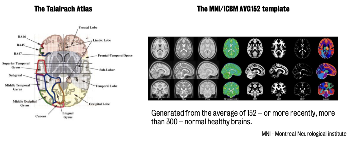
Two (2) most commonly used reference-based atlases:

• Talairach Atlas

  • Oldest

  • Based on the structure of a single individual who had suffered from a number of health problems

• MNI (Montreal Neurological Institute) Atlas

  • More commonly used

  • Is generated from the average of 152 (more recently >300) normal healthy brains.

Aligning the functional (T2) time series to the higher-resolution structural (T1) image is crucial before normalisation to standard space. This is because T1 images have better quality and lack the susceptibility artifacts common in T2 images, leading to more accurate normalisation parameter estimation.

• Normalisation of the T1 to standard space involves the initial affine registration of the images to get approximately the correct size and shape.

However, local variation in the distribution of brain tissue requires some local warping of the data that is facilitated by using non-linear warping parameters.

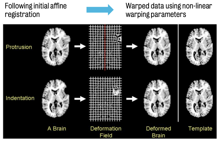
Mathematical functions (called discrete cosine transforms of increasing spatial frequency) can be combined to produce warped fields.

• These warp fields can be generated in all three axes, allowing for considerable flexibility and normalisation.

Part 2:

Smoothing involves the application of a filter to images in order to blur them.

• This filter is described in terms of its’ size, defined as the full width at half the maximum height (FWHM)

Smoothing of fMRI data:

① Increases signal-to-noise ration (SNR);

② Hides subtle errors in normalisation or anatomical variability;

③ Increases the normality of the errors/noise (linked to autocorrelation of residuals

④ Makes assumptions underlying Gaussian Random Field Theory (for multiple comparisons correction) that image smoothness is significantly greater than voxel size

As smoothing kernel size increases, the images become blurrier :. size of the smoothing kernel applied should be dictated by the size of spatial effect you'd expect to see

Data analysis

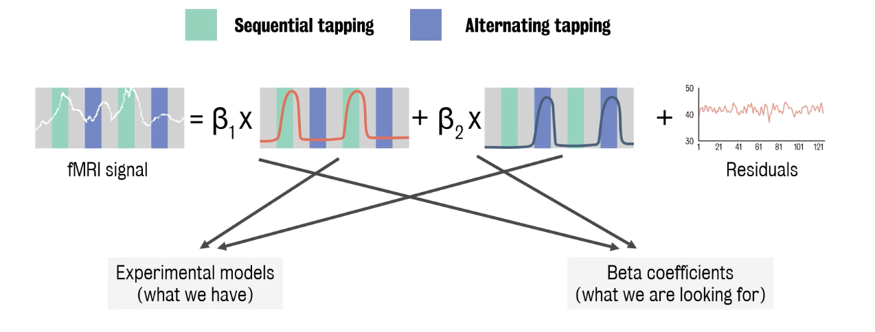
Observed data reflects linearly weighted sum of a collection of explanatory variables + some residual unexplained signal.

Shape of BOLD response depends on vasculature and varies across subjects (as well as across brain regions within one subject), and affected by drugs and aging.

High-pass filtering enhances images by removing low frequency information and leave high frequency information unchanged

Estimating beta parameter involves finding the values that minimize the sum of square error, i.e. minimize the mismatch between the weight of predictors and the data.

• Can be calculated by ordinary least squares, OLS, estimations,

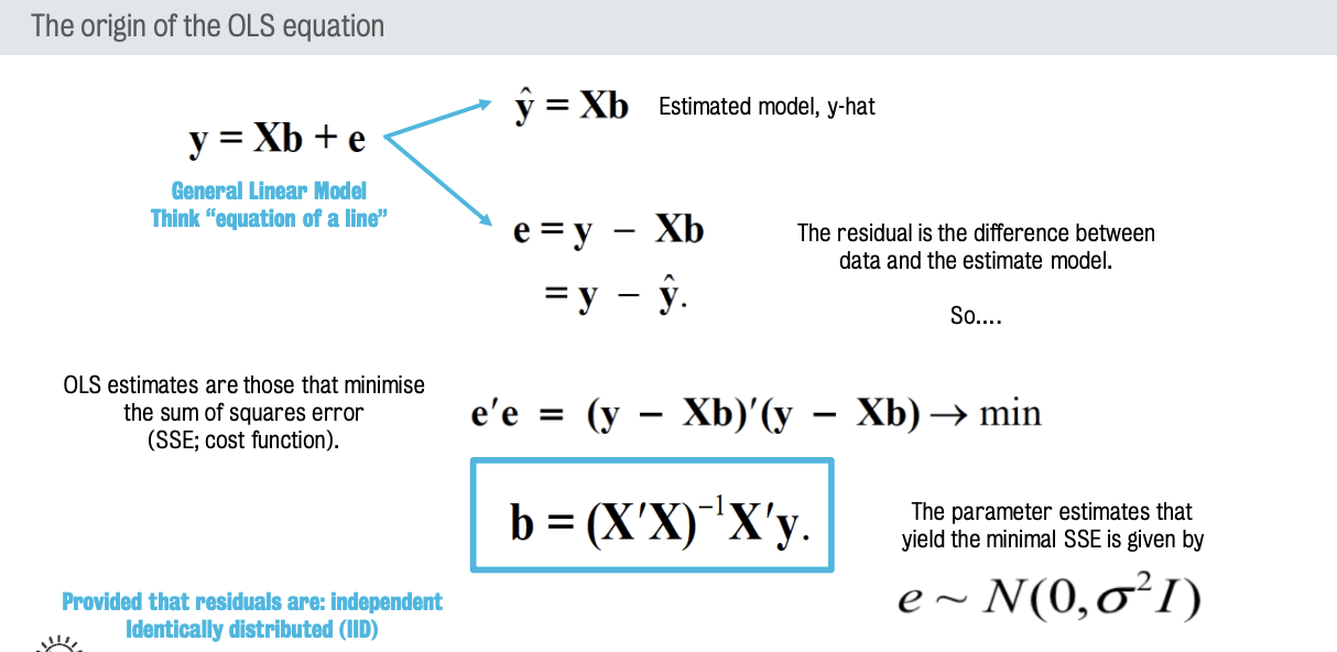
IID assumption suggests that if we take the residual (or error) from every time point in the time series and correlate them against one another, that the data points should be perfectly correlated with themselves, i.e. have a value of 1, but have no relationship with any other data points

To correct autocorrelation, we need to estimate the degree to which the data (or errors) explain observed error covariance.

• Correction for autocorrelation is typically referred to as pre-whitening of the parameter estimates, using a generalized or weighted parameter estimation rather than ordinary least squares.

Part 3:

Testing hypotheses and control for potentials false positives

In order to test hypotheses, we need to combine or compare regression coefficients, since model-fit parameters are our proxy for activation.

Analyzing constrasts:

Contrasts are linearly weighted sums of betas (regression coefficients) that permit the testing of specific hypotheses.

Contrast vectors are used to test specific hypotheses by combining or comparing beta parameters.

• For example, a contrast of [0, 1, -1] would test if the response to condition 2 is greater than the response to condition 3. This contrast is required to test whether there is a greater activation, ie a larger regression coefficient for condition 2 compared to condition 3, indicating the voxel is more responsive to stimulus 2 than it was to stimulus 3.

The contrast map (which represents the difference in the betas at every point in the brain) is then scaled with respect to the variance of the residual, ie the unexplained signal.

• This is equivalent to signal-to-noise ration and produces a statistical map with an associated p-value for every single voxel.

In mass-univariate analysis, each voxel is tested independently, leading to a high risk of false positives.

• Bonferroni Correction: A very conservative method for correcting for multiple comparisons by dividing the alpha level by the number of tests (voxels). This often leads to missing true effects (Type II errors).

There is considerable spatial correlation between voxel signals which arises from brain anatomy and other factors, including smoothing, which we add to the dat

Gaussian Random Field Theory (GRFT) is an approach to correct for familywise error (aka false positives) on the basis of truly independent tests in images.

• Accounts for the spatial correlation between voxel signals (due to brain anatomy, smoothing, etc.).

  • Estimates the number of "resolution elements" (resels) in the image, representing the number of independent tests. Then adjusts the p-value threshold based on the image smoothness to control the familywise error rate (FWER).

Expected Euler Characteristic (EEC) describes the number of clusters that appear on an image at a certain threshold

• GRF uses this mathematical function to predict the number of clusters that will appear on a statistical map at a given threshold. By setting the threshold to achieve a low expected Euler characteristic (e.g., 0.05), the probability of any false positive cluster is controlled.

Voxel-level correction applies the multiple comparisons correction at the individual voxel level, preserving spatial specificity.

Cluster-level correction ensures that the cluster as a whole is significant.

• First sets a cluster-forming threshold, then uses GRF to determine the minimum cluster size expected by chance given the image smoothness.

• ⚠ Only clusters exceeding this size are considered significant. While statistically powerful for detecting distributed activation, it reduces spatial specificity; the significance does not necessarily individual voxels within it.

Standard GLM-based fMRI analysis relies on assumptions like the IID nature of errors and the data approximating a smooth Gaussian random field.

• Outliers and non-independent errors can violate these assumptions, leading to inaccurate p-values.

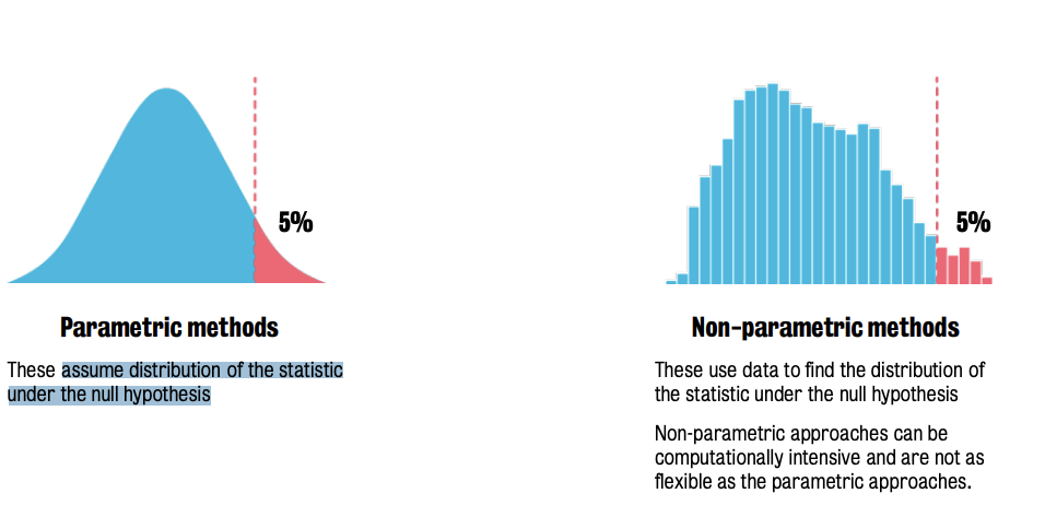
Increased interest in non-parametric approaches to image analysis in recent years.

• Methods like permutation testing are gaining popularity as they make fewer assumptions about the data distribution.

• These methods define the statistical distribution from the data itself.

• Computationally intensive and less flexible than parametric methods.

Meanwhile, parametric methods assume distribution of the statistic under the null hypothesis.

Key Terms:

• Affine Registration: A type of image registration that allows for translations, rotations, zooms, and shears, providing 12 degrees of freedom to align images.

• Autocorrelation: The correlation of a signal with a delayed copy of itself. In fMRI, it often refers to the dependence between error terms at adjacent time points in the time series.

• Blood-Oxygen-Level-Dependent (BOLD) Response: The change in magnetic resonance signal intensity that is sensitive to the level of deoxyhaemoglobin in the blood, which is indirectly related to neural activity.

• Bonferroni Correction: A conservative method for correcting for multiple comparisons by dividing the desired alpha level by the number of tests performed.

• Contrast: A vector of weights used in the GLM to test specific hypotheses by creating linear combinations of the estimated beta parameters.

• Coregistration: The process of aligning two or more images from the same subject that were acquired using different imaging modalities (e.g., structural T1-weighted and functional T2*-weighted images).

• Cost Function (Objective Function): A measure of the quality of alignment between two images, which is either minimized or maximized during the image registration process.

• Discrete Cosine Transform (DCT): A mathematical transformation used in fMRI analysis, often as a basis set for high-pass filters to model and remove low-frequency drift.

• Familywise Error Rate (FWER): The probability of making one or more false positive inferences across a set of statistical tests.

• Functional MRI (fMRI): A neuroimaging technique that measures brain activity by detecting changes in blood flow.

• Gaussian Random Field Theory (GRFT): A mathematical framework used in fMRI analysis to account for the spatial correlation in the data when correcting for multiple comparisons.

• General Linear Model (GLM): A statistical model used to analyze fMRI data by relating the observed BOLD signal to a set of explanatory variables.

• Haemodynamic Response Function (HRF): A model of the time course of the BOLD signal change in response to transient neural activity.

• High-Pass Filter: A signal processing technique that allows high-frequency signals to pass while attenuating low-frequency signals; used in fMRI to remove slow drifts in the signal.

• Independent and Identically Distributed (IID): A statistical assumption that data points are independent of each other and drawn from the same probability distribution.

• Mass-Univariate Analysis: A statistical approach used in fMRI where a separate statistical test is performed for each voxel in the brain.

• Motion Correction (Realignment): A preprocessing step that aims to correct for subject movement during fMRI scanning by aligning the different volumes of the functional time series.

• Montreal Neurological Institute (MNI) Atlas: A commonly used standardized brain atlas and coordinate system based on the average of many individual brains.

• Multiple Comparisons Problem: The increased chance of obtaining false positive results when performing a large number of statistical tests.

• Mutual Information: A measure of the statistical dependence between two random variables; used as a cost function for aligning images with different intensity characteristics.

• Normalization (Spatial Normalization): A preprocessing step that warps individual subjects' brains to match a standard template, allowing for group-level comparisons.

• Nuisance Regressors: Explanatory variables included in the GLM that are not of primary interest but are included to account for sources of noise or systematic variability (e.g., motion parameters).

• Ordinary Least Squares (OLS): A common method for estimating the parameters of a linear model by minimizing the sum of the squared differences between the observed and predicted values.

• Pre-processing: A series of initial steps applied to raw fMRI data to reduce noise, correct for artifacts, and prepare the data for statistical analysis.

• Resel (Resolution Element): A measure of the effective smoothness of an fMRI image, used in Gaussian Random Field Theory.

• Rigid Body Registration: A type of image registration that allows for only translations and rotations (six degrees of freedom), assuming the shape and size of the object remain unchanged.

• Signal-to-Noise Ratio (SNR): A measure of the strength of the desired signal relative to the background noise.

• Smoothing (Blurring): A preprocessing step that applies a filter (typically Gaussian) to fMRI images to increase SNR and reduce the effects of minor anatomical variations.

• Standard Space: A reference brain atlas and coordinate system used for normalization, allowing for comparison across individuals.

• Talairach Atlas: An older standardized brain atlas based on the anatomy of a single individual.

• T1-weighted Image: A structural MRI image with high contrast between grey and white matter.

• T2-weighted Image:* A type of MRI image commonly used for fMRI, sensitive to blood oxygenation levels.

• Voxel: The smallest unit of volume in an MRI image.