Lecture 2 - Introducing categorical predictors into a multiple regression model

Introduction to Categorical Predictors in Multiple Regression

• Focus on integrating categorical predictors into multiple regression models.

• A combination of theoretical understanding and practical demonstrations in R Studio.

• Availability of resources: ZIP file with slides and lab materials.

Model Overview

• Regression equation: Y = Intercept + Predictors + Error.

  • The fundamental regression equation can be expressed as:Y = Intercept + Predictors + Error. This informs us that a combination of its intercept value predicts the output variable (Y), the contributions made by various predictors, and random error.

• Interpretation of intercept: average value when continuous predictors are zero and categorical predictors are at reference levels.

  • The intercept represents the average expected value of the dependent variable (Y) when all continuous predictors are set to zero, and all categorical predictors are at their chosen reference levels. Understanding this can aid in accurately interpreting the regression outcomes.

• Continuous predictor interpretation: one-unit increase in predictor X changes Y by the beta coefficient.

  • For a continuous predictor, the interpretation of coefficients can be articulated as follows: a one-unit increase in predictor X will result in a corresponding change in Y by the beta coefficient associated with that predictor. This highlights the relationship and effect size of continuous variables on the dependent outcome.

• Categorical predictor interpretation: change from one group/level to another affects Y by the beta coefficient associated with that level.

  • When interpreting coefficients for categorical predictors, we understand that a change from one group or level to another influences Y by the beta coefficient linked with that specific level, emphasizing the comparative nature of categorical data.

Examples of Categorical Predictors

• Categorical variables with two levels:

  • Sex: Must be categorized as Female or Male.

  • Smoker Status: Either No or Yes.

  • Accuracy: Often evaluated binary as No or Yes.

  • Random Controlled Experiments typically involve comparison between Control and Treatment groups.

• Accuracy can also be binary: No and Yes.

• Random controlled experiments may have Control and Treatment groups.

Reference Levels in R

• The reference level is typically the category that appears first alphabetically or has the lowest numerical value upon data import.

• R's default contrast coding (dummy coding or treatment coding) manages binary predictors effectively, creating reference levels automatically.

• Importance of understanding reference levels:

  • Each coefficient describes the change in the outcome variable from the reference level to the specified level.

  • Reference level is embedded in the intercept, allowing easier interpretation of model outputs.

Data Preparation and Visualization

• Data loading in R:

  • Character variables: Sex, Smoker, Region.

  • Continuous variables: Age, BMI, Number of children, Insurance charges.

• Transform character variables into factor variables for analysis.

• Character Variables: Key categorical variables such as Sex, Smoker status, and Region.

• Continuous Variables: Factors including Age, BMI, Number of Children, and Insurance Charges. To conduct proper analyses, it's essential to transform character variables into factor variables, allowing them to be treated adequately in statistical models.

• Visualization of categorical variables reveals distribution:

  • Bar charts for categorical variables indicate even distribution for Sex and Region.

  • Correlation plots help understand relationships between continuous predictors.

  • Consider using dummy coding to represent categorical variables in the regression model, ensuring that each category is accurately reflected in the analysis.

  • The default contrast scheme in R for categorical variables is known as “Dummy coding” or “treatment coding”

    • 0 to a level 1

    • 1 to level 2

    • The level coded as 0 = variable reference level

    • Level that comes first in the alphabet / numerically

    • The reference level of a categorical variable is part of the Intercept term of a regression model

• Utilizing visual tools helps to unveil the distribution of categorical variables. For instance, bar charts effectively highlight the even distribution of categorical variables like Sex and Region, while correlation plots contribute to clarifying relationships between continuous predictors.

Model Fitting and Interpretation

• Setting up the regression model with six predictors.

• Model diagnostics include:

  • Overview of residuals.

  • High F-ratio and low p-value indicating good model fit and explained variance (75%).

• Coefficients interpretation:

  • Age leads to $256 increase in insurance; BMI leads to $339 increase; gender effects decrease charges by $130 for males; smokers face higher charges by $23,848 based on the region.

Changing Reference Levels

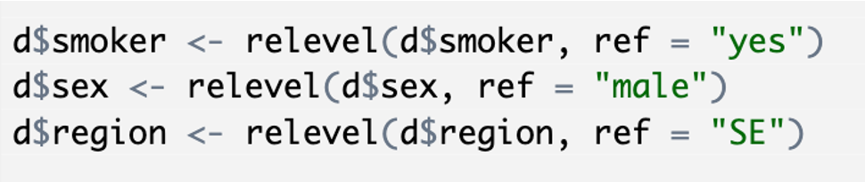
• Code provided to change reference levels for smoker status, sex, and region.

• Outcomes of changing reference levels change the interpretation:

  • The intercept may become positive and make financial sense.

  • Your hypothesis may mean a different reference level makes it easier to interpret

  • This may be useful in the context of factors with more than two levels

  • You can change the reference level by using the relevel() function to manually reorder the levels of your grouping variable

  • There are other ways too

    

Understanding Coding Schemes

• Dummy vs. Sum Coding:

  • Dummy coding reflects simpler contrasts between two levels.

    • This reflects straightforward contrasts between two levels of categorical variables, simplifying the interpretation.

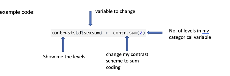
  • Sum coding centers categorical variables around zero, aligning with continuous predictors and useful for interactions.

    • This method centers the categorical variables around zero and is more aligned with the behavior of continuous predictors, making it useful for analyzing interactions.

• Processing more than two categorical levels:

  • Sum coding outputs differences from intercept, and models have coefficients reflecting these differences.

• Helmert Coding for Ordered Variables:

  • Difference between preceding levels is calculated.

  • Provides a staircase effect in coefficients.

Coefficient Interpretations:

The regression outputs reveal the following:

• For each additional year in Age, the insurance charges increase by approximately $256.

• For each unit increase in BMI, there's a corresponding increase of about $339 in charges.

• Gender effects suggest that males benefit from a decrease in charges by about $130 relative to females.

• Smokers face a significant increase in insurance charges amounting to $23,848, with variability based on region

Sum coding: preparing for inetractions

• Much better choice if you are including interactions in your regression model

• Instead of 0 and 1, -1 and +1 are used

• Intercept is now at 0

• Categorical predictor is now “centred” (explained later)

• Like continuous predictors

• This type of contrast can help for interpreting interactions that occur between categorical and continuous predictors

• Usually is half of the raw data

• nlike continuous predictors, categorical predictors are often represented using dummy coding, where each category is transformed into a binary variable, allowing for easier interpretation of their effects within the regression model.

Mean Centering and Standardization

• Mean centering provides a better understanding of the intercept:

  • It reflects the average participant rather than at zero.

  • Centred variables necessary for capturing natural data contexts.

  • Intecept shows average of scales

• Standardization allows comparison across continuous predictors by rescaling to a common measurement.

• This process involves centering continuous variables and dividing by the standard deviation.

• Additionally, when incorporating categorical predictors, it's essential to create dummy variables that represent the different categories, enabling their inclusion in the regression analysis.

• When you have an unbalanced binary categorical variable you have to find the main and then use that mean to adjust the coefficients accordingly, ensuring that the model accurately reflects the impact of the categorical variable on the dependent variable ie taking the mean away from every smoker sensitive variable

• Remember that the raw intercept term represents the average value when all predictors are at zero

• So the coefficients are interpreted as the change in Y for some value (larger than 0) the X predictor

• An Intercept like this often doesn't make sense for the verbal model, i.e. the research questions or our hypotheses

• What does an intercept term of 0 years or 0 kgs mean?

• If we mean-centre the continuous predictors, the Intercept now represents the average value when all continuous predictors are at their average value

• Subtract the mean value of a variable from every observation in that variable

• The mean of the variable is then = 0

• All values are “centred” around zero

• Some will be below zero, some will be above

• The intercept term in your model now represents the intercept at the average for the predictor

The predictors are still in their raw units (e.g. years / kgs)

(learn to do these techniques by hard coding – easy to do and the common function that is used (scale()) doesn’t play very nicely with some other packages!)

Diagnostic Checks and Reporting

• Residual checks for model fit; clusters indicate potential interactions might be required.

• Data summary needs descriptive statistics for continuous variables and frequencies for categorical variables.

• Importance of p-values in identifying significant predictors and preparing for results reporting, adhering to APA standards.

• Monitoring residuals is essential to evaluate model fit, with clusters indicating the potential necessity for interaction terms. The data summary should always encompass descriptive statistics for continuous variables and frequency counts for categorical variables. The assessment of p-values remains critical for pinpointing significant predictors, aiding in the preparation of results reporting following APA standards.

Standardisation

• Take your centred variable and divide each observation by one standard deviation of the variable

• Interpretation is now a one standard deviation decrease / increase in the predictor is a (part of) standard deviation in the outcome variable.

• Because all predictors are now measured in standard deviation units, instead of their raw units, you can compare the size of their coefficients. You couldn’t do this before because they were in different units.

• Dividing by 2 standard deviations allows you to directly compare the coefficients for continuous and binary predictors.

• Standardization allows comparison across continuous predictors by rescaling to a common measurement.

More than 2 levels

- What about categorical variables with more than two levels?

• Dummy / treatment coding - each level’s coefficient is the difference between the reference level and one other level

• Sum coding – each level’s coefficient is the difference of the level from the intercept

• In variables with more than one level, To find the value of -1 , you have to calculate the sum of the intercept and all the other levels of the variable. – demonstrated earlier

• When working with categorical variables that feature more than two levels, sum coding generates outputs representing deviations from the intercept, leading to coefficients that reflect these deviations in a meaningful way.

Oredred variables

• Ordered outcome variables use ordinal regression model (week 19)

• Ordered predictor variables use “helmert” contrast coding

• Each level of the coefficient is the difference between those level or levels below them

  To get the value of the nth level in an ordered variable, you add all the other coefficients that come before that level to the intercept.

Summary: dummy coding

• Reference level in dummy coding becomes hidden in the intercept for the categorical predictor

• It’s a good idea to write out what your intercept represents before you start to interpret your model

• If dummy coding is used, switching from one level of the categorical predictor to the second level is the same as moving along one unit of a continuous predictor

• It follows that for a binary categorical predictor, the slope term is giving you the mean difference between the two groups.

  

Summary: Sum coding

• Intercept now reflects 0 rather than the reference level

• If sum coding is used, switching from one level of the categorical predictor to the second level is the same as moving along two units of a continuous predictor

  • compared to the raw model, binary variable coefficients will be half the size

• For variables of more than two levels, you need to add all the coefficients in the model summary together to find the coefficient for the -1 variable

Summary: standardised variables

• Centre a predictor and then divide the observation by the standard deviation of the variable

• Great for preparation for a model with interactions

• Each standardized variable now predicts the change in the outcome variable for a one standard deviation increase in the predictor variable

• Each standardized variable can now be compared with each other – allowing for judgements about relative strengths of predictors

Summary: Helmert contrasts for ordered variables

• Ordered predictor variables use “helmert” contrast coding

• The first coefficient is the change in Y for the difference between the first two ranks or levels of the variable

• The next coefficient is the change in Y for that specific level and the first two levels put together

• The next coefficient is the change in Y for that specific level and the first three levels put together

  …and so on

Conclusion and Further Applications

• Categorical predictors in regression require careful consideration of coding schemes and interpretations.

• Standardization helps compare the strength of predictors in terms of influence on outcomes.

• Future labs will delve into applying these concepts more broadly.

Introduction to Categorical Predictors in Multiple Regression

This segment focuses on the integration of categorical predictors into multiple regression models, which is crucial for understanding how different types of data influence outcomes in a statistical context. The learning experience combines theoretical foundations with practical demonstrations executed in R Studio, a powerful tool for statistical analysis and data visualization. Additionally, resources including a ZIP file containing slides and lab materials are readily available to support this learning experience.

Reference Levels in R

The reference level plays a pivotal role in regression analysis, often being the first level in alphabetical order or the level with the lowest numerical value upon data import. R effectively employs default contrast coding (also known as dummy coding or treatment coding) which manages binary predictors automatically, establishing reference levels as required. Understanding the significance of reference levels is crucial, as each coefficient in the model elucidates the change in the outcome variable concerning the reference level, and this is thoroughly embedded in the intercept, enhancing the interpretability of model outputs.

I