Week 11 - ECMT1020: Introduction to Econometrics - Chapter 7: Heteroskedasticity

Homoskedasticity

Our assumption of regression before is the disturbance term being homoskedastic (constant).

• Assumption of "constancy of variance" is crucial in homoskedasticity.

  • Model:

    

  • Assumptions:

    

• Error term is assumed to drawn from the same probability distribution.

  • This assumption often fails in practice, especially when individual characteristics influence outcomes (e.g., household expenditure vs. income).

• Homoskedasticity

  • Observations without error term represented by a solid line.

    

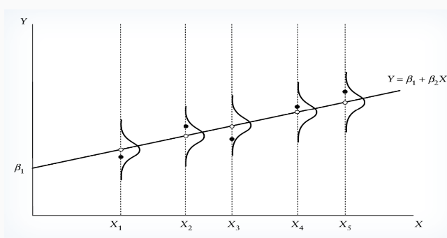
  • Disturbance term shifts the realized value of Y.

  • Probability of error term realization is identical across samples.

  • Homoskedasticity concerns consistent dispersion for all observation:

    

Heteroskedasticity

Heteroskedasticity refers to the circumstance in regression analysis where the variance of the errors is not constant across all levels of the independent variable(s). This can lead to inefficient estimates and affect the validity of statistical tests.

• heteroskedasticity does not affect unbiasedness.

• Homoskedasticity is required to make OLS BLUE (best linear unbiased estimator)

• Heteroskedasticity Characteristics

  • Probability of error term realization may depend on the size of X.

    

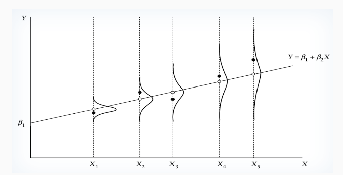
  • Variance of error term:

    

  • Heteroskedasticity likely to be problematic when variable values vary significantly across observations.

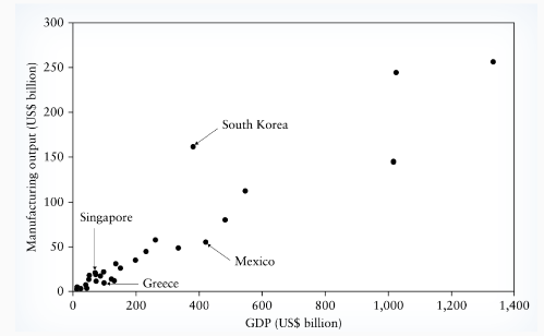
• Similar GDPs (e.g., South Korea vs. Mexico) can yield different manufacturing outputs due to sector importance.

Heteroskedasticity Impact on variance of OLS estimator

• Impact on OLS Estimates

  • Normal variance of OLS estimator only assumed to work with homoskedasticity, won’t work if heteroskedasticity is present.

    

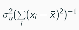
  • Misspecification in variance (equation above) can lead to incorrect statistical conclusions (t-tests, F-tests).

    

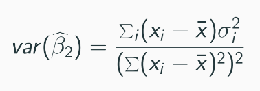
  • Variance formula changes, making standard t-statistics based on homoskedasticity assumptions incorrect, so that it can work under influence of heteroskedasticity.

The aftermath of the change in equation

The OLS estimator remains unbiased and consistent even with heteroskedasticity, but it loses efficiency. This means that while the estimates are still valid, the standard errors calculated under the homoskedasticity assumption will not accurately reflect the true variability of the estimates, leading to potentially misleading inferences.

To address this issue, robust standard errors can be used, as suggested by White (1980), which allows for consistent estimation of the variance of the OLS estimator in the presence of heteroskedasticity.

However, even with robust standard errors, the OLS estimator is still less efficient compared to the generalized least squares (GLS) estimator, which has a smaller variance.

• Generalized Least Squares (GLS) provides a linear unbiased estimator with smaller variance.

Detection of heteroskedasticity: Goldfeld–Quandt Test

• Detection of Heteroskedasticity: Goldfeld–Quandt Test

  • Assumes variance of error term is proportional to size of X.

  • Assume the error term is normally distributed.

  • Testing Procedure:

    1. Order observations by size of X and divide into 3 groups: group 1 with n*, group 2 with n-2n*, group 3 with n*

    2. Regress first and last groups to obtain RSS1 and RSS2 (exclude the middle group completely).

    3. Compute test statistic:

       

       k is the no. of parameters in regression model

  • Under null hypothesis of homoskedasticity, RSS₂ is not greater than RSS₁, and there is no heteroskedasticity in the disturbance term, or the disturbance term is homoskedastic.

    

Note: we take the larger RSS divided for the smaller one! To ensures the test statistic is always greater than or equal to 1, which aligns with the F-distribution's properties. Or else, wouldn’t work against comparing critical value.

Steps in STATA:

• sort X

• reg Y X in 1/n*

• reg Y X in n-n*+1/n

• then manually calculate F = RSS2/RSS1

Results:

The power of test depends on the choice of n* relative to n.

GQ suggests n* approx 3n/8.

Under the null of homoscedasticity (heteroskedasticity presents and the variance depends on the value of X_i), RSS₁ and RSS₂ would be different from each other’s, RSS₃ would be larger than RSS₁.

X_i is the variable expected to generate heteroskedasticity in the model.

If variance is inversely proportional to the size of X_i, test statistic will be replaced by RSS₁/RSS₂.

Detection of Heteroskedasticity: White Test

Test procedure

• Detection of Heteroskedasticity: White Test

  • Uses residuals as a proxy for disturbance term.

  • Testing Procedure:

    1. Compute residuals from OLS estimates.

       

    2. Regress squared residuals u^² on X and X² (think of residual now the dependent variable, a new regression equation)

    3. Compute test statistic nR²

  • Under null hypothesis:

    

    where variance of u is constant and does not depend on X.

We allow the variance of errors to be some flexible function of explanatory variables:

• the null hypothesis is to be tested is all coefficients above are 0 and the F test can be used to test the null.

Steps:

1. estimate the model using OLS

   

2. Calculating the squared residual, the fitted value and squared fitted value

   

3. Run the egression of squared residual and keep this from the regression

   

4. Calculate F-statistic

   

Alternatively, we can use LM statistic nR²_u² and compare it with critical value in X₂² distribution (Stata: estat imtest)

Steps in STATA

1. predict Y, resid

2. gen YSQ = Y*Y

3. gen XSQ = X*X (and so on)

4. gen XY = X*Y (and so on)

5. reg Y X Z …

6. estat imtest, white

The rationale behind using the squared residuals (step 2)

The rationale behind using the squared residuals is that heteroskedasticity implies that the variance of the error term is not constant but varies with the independent variable(s).

• By regressing the squared residuals on X and X², you can identify whether there is a systematic relationship between the independent variable(s) and the variance of the residuals. If the regression shows significant results, it indicates that the variance of the errors is related to the values of X, thus suggesting the presence of heteroskedasticity

Effect of number of regressors on the residual

If there are more than 2 variables, include their interaction terms and squares together as additional covariates.

• e.g. if there are 4 regressors, p = 15 (use explanation on the lecture slide)

Remedies for heteroskedasticity

Approach 1

• Approach 1: Infeasible Generalized Least Squares (Weighted Least Squares)

  • If ( E[u^2_i] = sigma^2_i ), scale the model by ( 1/sigma_i ).

    

  • New error term has mean 0 and variance 1.

  • GLS estimator is better estimation compared to standard LS estimator under heteroskedasticity.

The parameters of interest in the transformed model can be estimated by minimizing RSS:

where 1/σ² can be understood as the weight in the optimization problem:

• we give larger weight to the observation that involves smaller uncertainty.

Approach 2

• Remedies for Heteroskedasticity

  • Approach 2: Proxy-based Weighted Least Squares

    • If ( \sigma_i = \lambda z_i ) (where ( z_i ) is independent of ( u_i )), correct heteroskedasticity by using ( y_i/z_i ) and ( x_i/z_i ).

      

    • This method relates to the Goldfeld-Quandt test assumption, STD is proportional to X.

Robust Standard Errors

• Robust Standard Errors

  • OLS can be unbiased and consistent even with heteroskedasticity, but efficiency is compromised.

    

    Variance of OLS estimator is RHS below if u_i is independent across i

    

• White (1980) suggested replacing ( \sigma^2_i ) with ( \hat{u}^2_i ) for consistent variance estimation.

  • This method relies on asymptotic theory, which may not perform well in finite samples.

Consequence of heteroskedasticity

• Consequence of Heteroskedasticity

  • Example model:

    

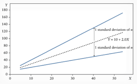
    Heteroskedasticity gets bigger as X values gets bigger.

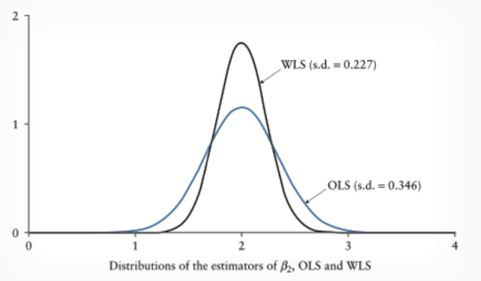
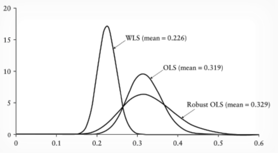
• Distributions of Estimators

  • Comparison of OLS and WLS estimators shows differences in standard deviations and means.