AP Statistics Final 🥑

Unit 1:

Displays of Data

• Bar Graph (categorical)

  • Each bar represents the frequency (counts) or relative frequency (percent) for each category

  

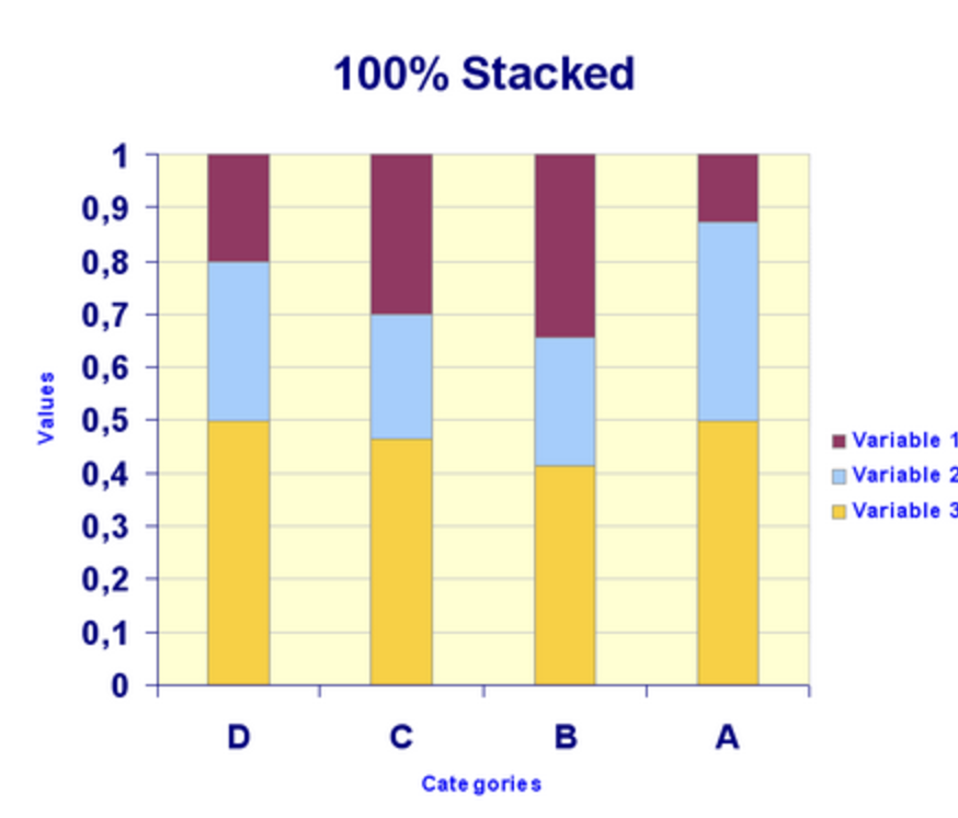
• Segmented Bar Graph

  • Stack the bars to make 100%

    

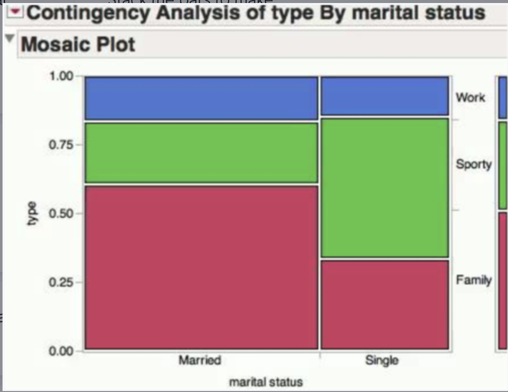
• Mosaic Plot

  • A segmented bar graph where the width of the bar is proportional to the size of the group.

    

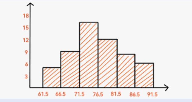
• Histogram (Quantitative)

  • a chart that plots the distribution of a numeric variable's values as a series of bars

  

• Stem Plot

  • Steps:

    • 1. Sort the data: Put the numbers in order from least to greatest.
      
      2. Identify the stems: Decide which digits will be the stems and which will be the leaves. The stems are the first digits of the numbers, and the leaves are the last digits.
      
      3. Draw the plot: Create a t-chart with a vertical line down the middle and a column on the left for the stems and a column on the right for the leaves.
      
      4. Add the stems: List the stems in the stem column in order from least to greatest.
      
      5. Add the leaves: For each stem, add the leaves in numerical order to the right.
      
      6. Create a key: To help the reader understand the plot, create a key that explains what each value represents. For example, you can write 6|8=68 to show that 6|8 represents 68.

    

    • How to tell skewness from a stem and leaf plot

      

• Box & Whiskers Plot

  • A standard "box and whiskers plot" displays the full range of data within the whiskers

  • Modified Box & Whiskers Plot

    • A "modified box and whiskers plot" adjusts the whiskers to explicitly identify outliers by only extending them to a calculated point based on the interquartile range

    • How to make modified

      • *Calculate outliers & remove from data set, then re-calculate the 5 number summary and graph

        

Variables

• Categorical variables

  • A categorical (or qualitative) variable takes on values that are category names or group labels.

    

• Quantitative Variable

  • A quantitative variable takes on numerical values for a measured or counted quantity.

    • 2 types of quantitative variable:

      • discrete quantitative variable - takes on a finite or countable number of values. (e.g., only whole numbers)

      • continuous quantitative variable can take on uncountable or infinite values with no gaps, such as heights and weights of students. (e.g., out to an infinite number of decimal places).

• Vertical axis manipulation

  • a technique used to make a graph misleading by altering the scaling of the y-axis

  

• Flaw with pictographs

  • They generally do not follow the area principle.

    ---

• Explanatory Variable

  • a variable that we think explains or causes changes in the response variable

• Response Variable

  • The value is measured or recorded. It is a quantitative value.

Two Way Table & Relative Frequencies

• Two Way Table

  • A statistical tool used to display the frequency of data where two categorical variables are being analyzed, with one variable represented by the rows and the other variable represented by the columns

    • Marginal relative frequency from a two way table

      • divide the frequency of a row or a column total by the total frequency
        

        

        
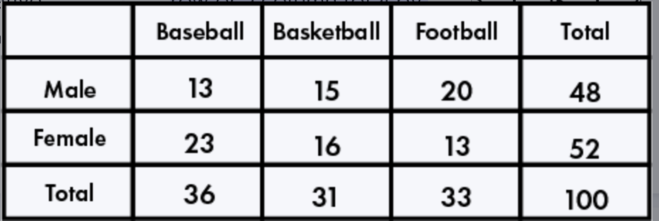
        ex. 31/100

    • Joint relative frequency

      • divide the frequency within a specific cell (not in the total row or column) by the grand total number of observations in the table

        

        ex. 15/100

    • Conditional relative frequency

      • divide the joint frequency of a specific category within a given condition (row or column) by the marginal frequency of that condition (the total count for that row or column) in a two-way frequency table

        

Association

• Association

  • Knowing the value of one variable helps us predict the value of the other variable.

    • What happens if two variables are associated?

      • The segmented bar charts look different.

• An association between variables?

  

• NOT an association between variables?

  • The bars will look approximately identical

  • No association means _________.

    • Proportion should remain the same

SOCV

• SOCV

  • shape, outliers, center, variability

    • use SOCV to describe distribution

  • Shape

    • skewed left, skewed right, symmetric (unimodal), bi-modal

      

    • Difference between Unimodal & Symmetric

      • No, "unimodal" and "symmetric" are not the same thing in statistics; while a unimodal distribution has only one peak, a symmetric distribution is one where the data is evenly distributed on either side of the center point

  • Outliers

    • Any potential outliers

    • How to calculate outliers?

      • By doing the 1.5 X IQR Test:
        
        For the low outlier: way to small < Q1 - 1.5(IQR)
        
        For the big outlier: way to big < Q3 + 1.5(IQR)

    • How to calculate IQR?

      • Q3-Q1

    • What are affected by outliers?

      • Mean and SD

    • What is NOT affected?

      • Median and IQR

  • Center

    • Mean:

      • if the data is symmetrical and has no outliers. you can check this by seeing if the mean and median are approximately same.

        • EX: "The mean would be the most appropriate measure of center as the distribution is roughly symmetric.”

    • Median

      • when your data is skewed (not symmetric) or contains outliers

        • EX: "The median would be the most appropriate measure of center as the distribution is skewed left."

  • Variability

    • Write the range (Max-min) and the standard deviation

• 5 Number Summary

  • min, Q1, median, Q3, max

Standard Deviation

• Standard Deviation:

  • the square root of the variance. The standard deviation gives a typical distance that each value is away from the mean.

• Golden sentence when you are told to interpret the value of the Standard Deviation?

  • "The (insert context) typically varies by the value of the (insert standard deviation) from the mean of (insert mean).
    
    Example: "The annual rainfall for these 9 cities typically varies by the value of 15.52 inches from the mean of 34.94.

• More Variation

  • Higher SD

Unit 2:

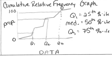
Percentile & Cumulative Relative Frequency

• Interpreting percentile

  • “(the pth percentile/percent) of [insert context] are at or below [insert that value]”

• Cumulative Relative Frequency Graph

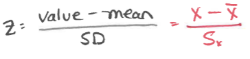
Z-Score

• Z-scores measure standard deviations from the mean.

  • Show positive relative from the mean in a distribution

  • They standardize the distribution

  

• Golden Sentence:

  • “Insert Context is z-score standard deviations above/below the mean of x̄.”

Normal Distribution Calculations

• Normal distribution

  • provides a valuable model for how many sample statistics vary, under repeated random sampling from a population.

• Calculations involving normal distributions are often made through z-scores

  • z-scores measure standard deviations from the mean.

• On the TI-84:

• normalcdf(lowerbound, upperbound) gives the area (probability) between two z-scores

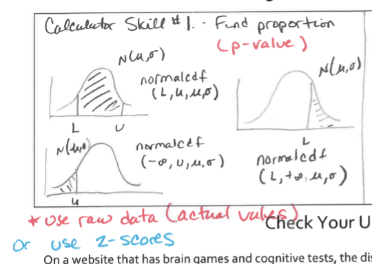
• invNorm(area) gives the z-score with the given area (probability) to the left.

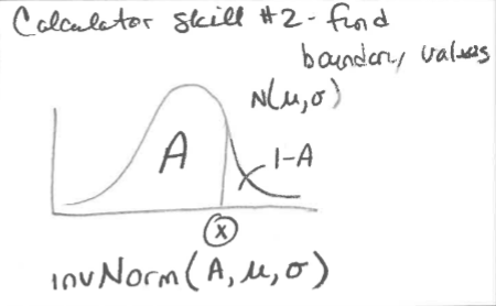
• The TI-84 also has the capability of working directly with raw scores instead of z-scores. In this case, the mean and standard deviation must be given:

To receive full credit for probability calculations using the probability distributions, you need to show:

1. Name of the distribution ("normal" in the example above)

2. Parameters ("µ = 1500, σ = 75" in the example above)

3. Boundary ("1410" in (a) of the example above)

4. Values of interest ("<" in (a) of the example above)

5. Correct probability (0.1151 in (a) of the example above)

The Normal Distribution/Bell Curves/Density Curves

• Normal distribution is valuable for providing a useful model in describing various natural phenomena. It can be used to describe the results of many sampling procedures.

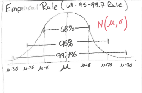
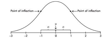
• The normal distribution curve is bell-shaped and symmetric and has an infinite base.

• The mean of a normal distribution is equal to the median and is located at the center. There is a point on each side where the slope is steepest. These two points are called points of inflection, and the distance from the mean to either point is precisely equal to one standard deviation. Thus, it is convenient to measure distances under the normal curve in terms of z-scores.

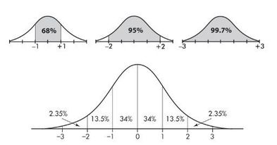
The empirical rule (also called the 68-95-99.7 rule) applies specifically to normal distributions. In this case, about 68% of the values lie within 1 standard deviation of the mean, about 95% of the values lie within 2 standard deviations of the mean, and about 99.7% of the values lie within 3 standard deviations of the mean.

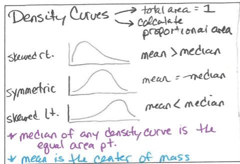
• Density Curves

  • 

Linear Transformations of Data

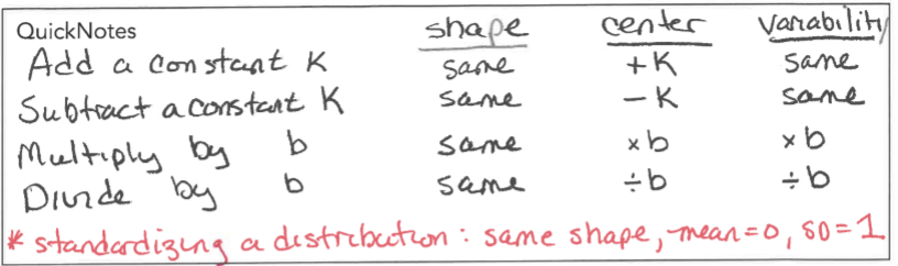
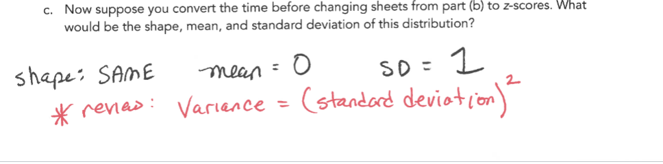
** Z-SCORE DOESNT CHANGE

MEAN = 0, SD = 1

Unit 3:

Scatterplots

• Describe a Scatterplot

  • DUFS

    • Direction (positive,negative,none)

    • Unusual Features (outliers,high lev. point)

    • Form (roughly linear, non-linear)

    • Strength (strong, moderate, weak)

  • Golden Sentence:

    • Ex. “There is a weak, negative, roughly linear, and one possible outlier between screen time & rank”

Correlation

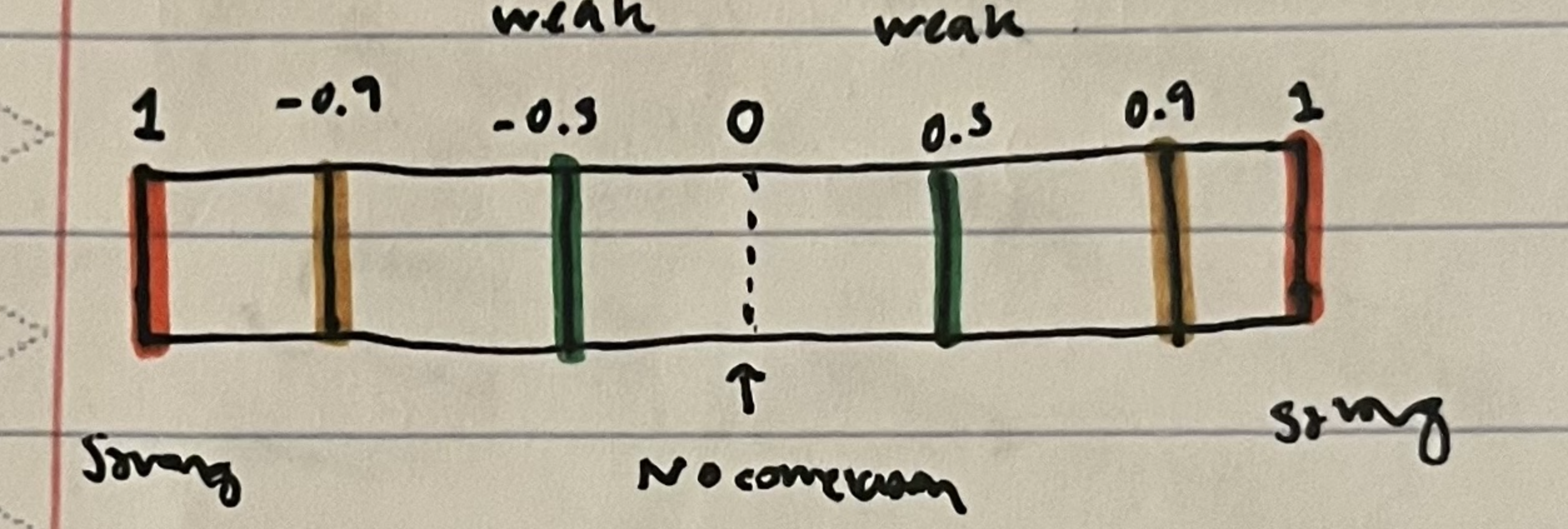
• Golden Sentence: Interpret Correlation (r)

  • The linear relationship between explanatory variable(x) & response variable(y) is strength and direction.

    • ex. r=0.987

      • The linear relationship between number of rubber bands and distance travelled is strong and positive

• Golden Sentence: Interpret Coefficient of Determination (r²)

  • r^2% of the variation in y(response) can be explained by the linear relationship with x(explanatory).

    • ex. r²=0.974

      • 97.4% of the variation in distance travelled is explained by the linear relationship with the # of rubber bands.

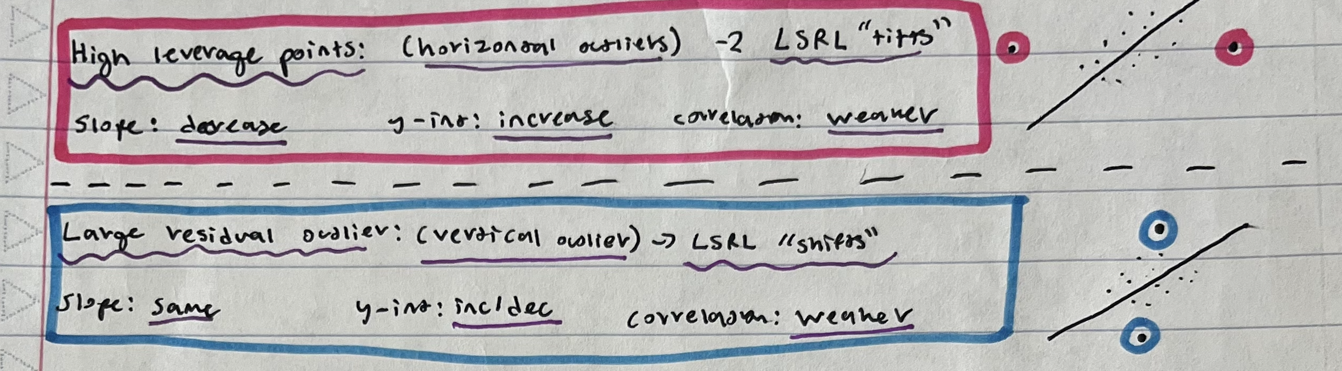
Types of Outliers & Causation/Correlation

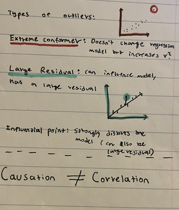
• Why are outliers considered outliers?

  • They DO NOT follow the overall trend (or large residuals)

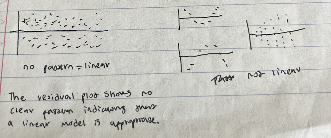
Regression & Residuals

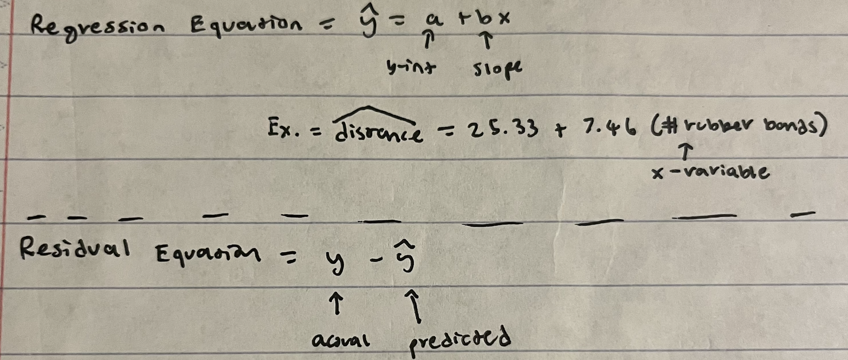
• Golden Sentence: Interpretation of y-intercept

  • The model predicts a context of y-int when x=0

    • ex. The model predicts that Michael burns 20 calories when he runs 0 miles.

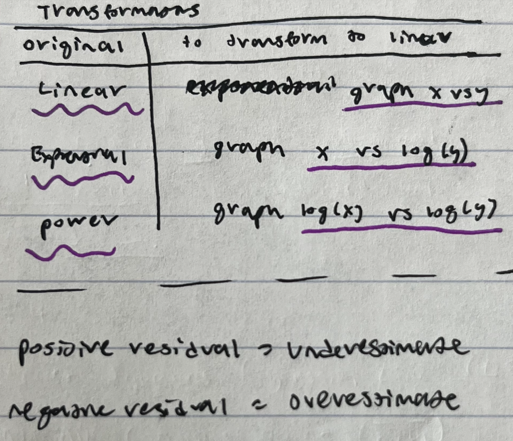
• Golden Sentence: Interpretation of residual

  • The actual y was residual above/below the predicted value of x=____. 

• Golden Sentence: Interpretation of slope

  • The model predicts an increase/decrease of slope for each additional unit of x. 

    • ex. The model predicts an increase of 160 calories for each additional mile Michael runs.

• Extrapolation

  • Infer the unknown from the known (make a prediction)

    • It is often inaccurate!!!

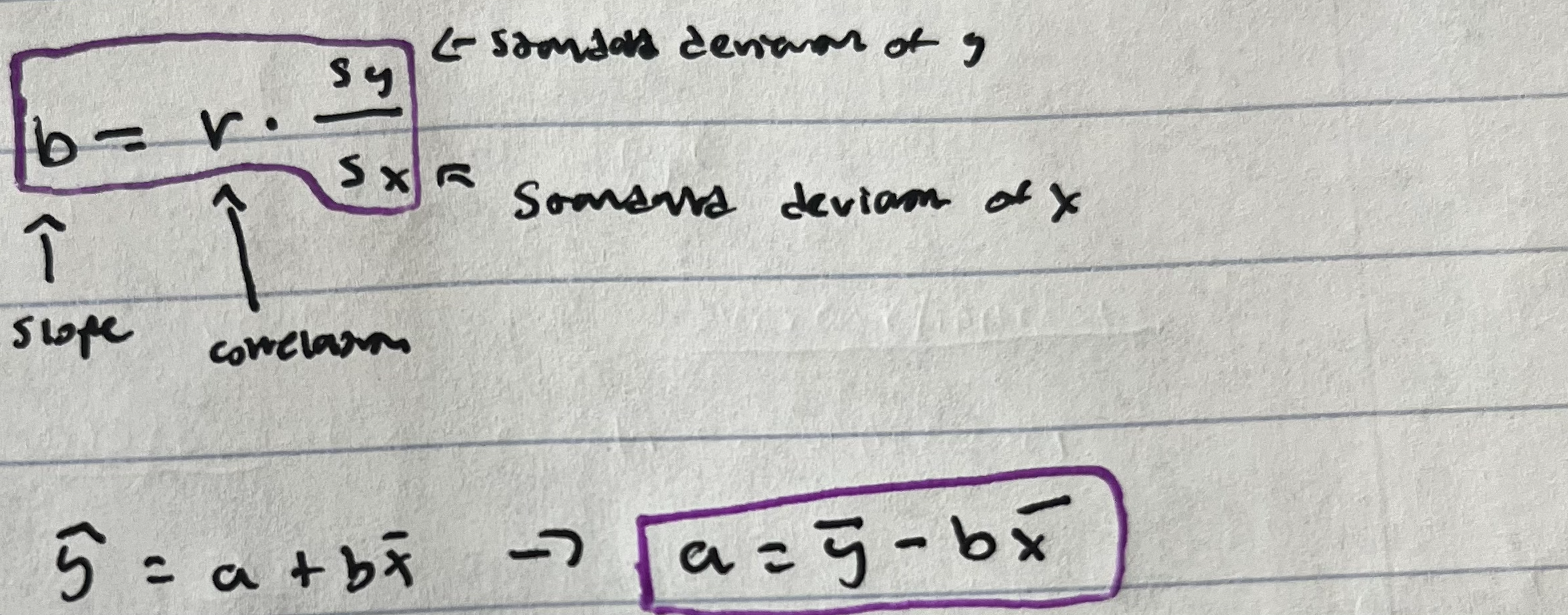
• Least Squares Regression Line (LSRL)

  • The LSRL minimizes the sum of the square residuals

    • The “best” best fit line

    • ALWAYS contains point (x̅, ȳ)

    • 

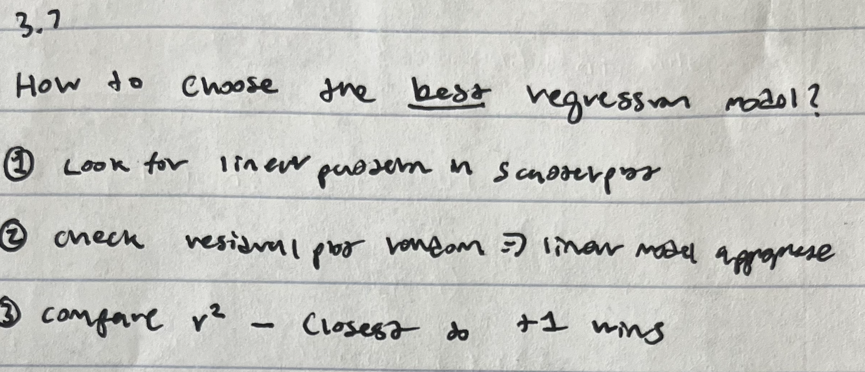
• How to choose the best regression model

  • 

• Equations

  

Points

High Leverage Points/Large Residual Outliers

Transformations

Unit 4:

Sampling: 💚

Convenience sample:

• are based on choosing individuals who are easy to reach.

• tend to produce data highly unrepresentative of the entire population.

  → how does it lead to bias?

  • it selects participants based on their availability rather than a random selection

Voluntary Response Sample

• individuals who choose to participate

• gives too much emphasis to people with strong opinions

• undersamples people who don’t care much about a topic

  → how does it lead to bias?

  • leads to bias as only people w strong opinions (usually negative) will respond

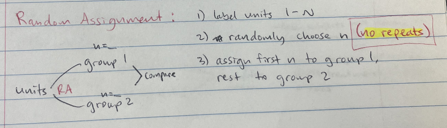
Simple Random Sample

• every possible sample of the desired size has an equal chance of being selected

  → how does it lead to bias?

  • if the sampling frame (the list of potential participants) does not accurately represent the whole population

• Process:

  1. label individuals 1-#

  2. use a random number generator to select a # of them

  3. select and survey respondents (no repeats)

     "randomization reduces bias"

Stratified Random Sample

• dividing the population into homogeneous groups called strata

  • homogenous: very same or similar

• then pick random samples from each of the strata

  

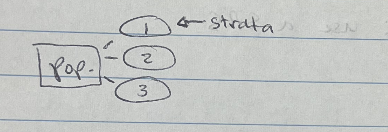
• finally combining these individual samples into a stratified random sample

  • For example, we can stratify by age, gender, income level, or race; pick a sample of people from each stratum; and combine to form the final sample.)

• low variability

• low bias

  → how does it lead to bias?

  • if the sampling frame (the list of potential participants) does not accurately represent the whole population

Cluster Sample

• involves dividing the population into heterogeneous groups called clusters and then picking everyone or everything in a random selection of one or more of the clusters.

• For example, to survey high school seniors, we could randomly pick several senior class homerooms in which to conduct our study and sample all students in those selected homerooms.

  → how does it lead to bias?

  • when the selected clusters are not representative of the overall population, leading to an over- or under-representation of certain subgroups within the sample

Systematic Random Sample

• listing the population in some order (for example, alphabetically), choosing a random point to start, and then picking every tenth (or hundredth, or thousandth, or kth) person from the list.

  → how does it lead to bias?

  • if the population list is ordered in a way that creates a repeating pattern, leading to the over-representation of certain subgroups within the sample

Bias: 🥶

1. Undercoverage bias - happens when there is inadequate representation, and thus some groups in the population are left out of the process of choosing the sample.

2. Response bias - describing situations where people do not answer questions truthfully for some reason. people don’t want to be perceived as having unpopular or unsavory views or don’t want to admit to having committed crimes.

3. Nonresponse bias - when individuals selected to be in the sample who do not respond to the survey have different opinions from those who do.

   1. Nonresponse bias has no volunteers, its just selects people who don’t respond

4. Convenience Sample Bias - As the sample is based on people who are willing at the time and place that the researcher is present, you won't be gaining a range of people each time you're collecting data.

5. Voluntary Response Bias - occurs when a sample of people is chosen to participate in a survey by their own choice, rather than being randomly selected. This can lead to biased results that are not representative of the entire population.

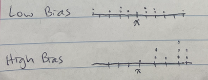
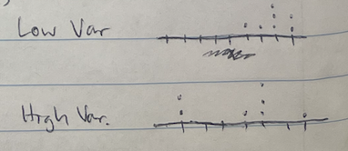
What does low vs high bias look like on a dot plot??

What does low vs high variability look like on a dot plot??

Calculator Functions: 😚

randint( 1, 10, 2)

(Domain,How many random #’s)

Example:

1. label the seats 1-50

2. use randint(1,50,10)

3. ignore & replace repeats

4. select & survey people in corresponding seats

Study Types + Treatments: 😌

Census : Collecting data from every individual in a population. Downfalls of this method: expensive, time consuming.

Observational Study: No treatment is imposed; observational studies aim to gather information about a population without disturbing the population.

Observational studies NEVER establish cause & effect!!!!!!

Experiment: Treatment is imposed

Prospective Study: individuals are followed over time and data about them is collected as their characteristics or circumstances change.

Retrospective Study: involves analyzing data that has already been collected to answer a scientific question. observational studies by necessity because they assess past events and it is impossible to perform a randomized, controlled experiment with them.

Statistically Significant: the difference between the two is large enough that you can say it wasn’t by chance

The Language of Experiments: 🤑

• Experimental units - An experiment is performed on objects.

• Subjects - If the units are people.

• Experiments involve explanatory variables, called factors, that are believed to have an effect on response variables. A group is intentionally treated with some level of the explanatory variable, and the outcome of the response variable is measured.

• Elements of a Well-Designed Experiment:

  • Comparison (2+ treatment groups)

  • Random assignment

  • Replication (more than 1 unit in each treatment group)

  • Control (Keep other variables constant)

• Placebo Effect - It is a fact that many people respond to any kind of perceived treatment. (For example, when given a sugar pill after surgery but told that it is a strong pain reliever, many people feel immediate relief from their pain.)

  • Placebos are used primarily for blinding

  • A treatment that has no active ingredients

• Blinding - occurs when the subjects don’t know which of the different treatments (such as placebos) they are receiving.

• Double-blinding - is when neither the subjects nor the response evaluators know who is receiving which treatment.

• Experiment: Treatment is imposed, allows causation

• Treatments: What is done/not done to experimental units

  • Replication of the treatments on many units reduces the role of chance variation.

    • by repeating an experiment on a large number of different units (individuals, samples, etc.) under the same treatment conditions, the influence of random, unpredictable variations ("chance variation") on the results is minimized, allowing for a more accurate assessment of the true effect of the treatment itself. 

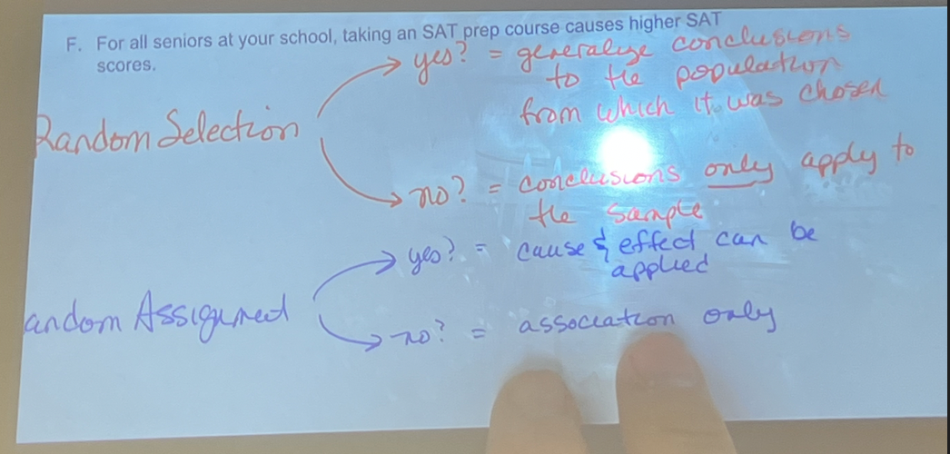
Randomization: 🥰

• Random selection: generalize conclusion to the population (BIG)

  • IF NOT USED, generalize conclusion to the sample (smol)

• Random Assignment: Cause (MENTION CAUSED!!!) & effect can be applied

  • IF NOT USED, association can be applied

Ex. Random selection (Yes), Random Assignment (No)

For those at Wisconsin, there is an association between volunteering and decreased mortality rates

• Random Assignment:

  

Random Selection & Random Assignment:

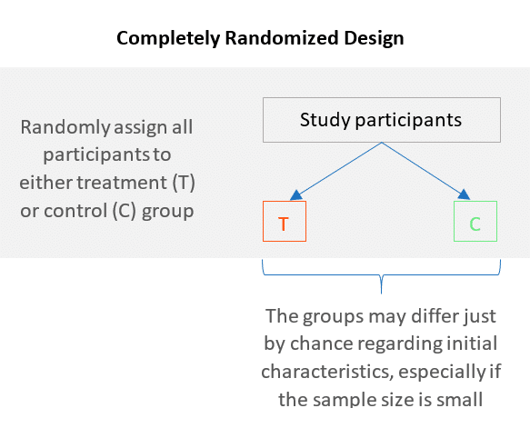
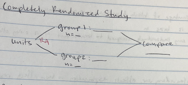
Design: 💝

• Completely Randomized Design/Study: Randomly assign all participants to either treatment or control group

  

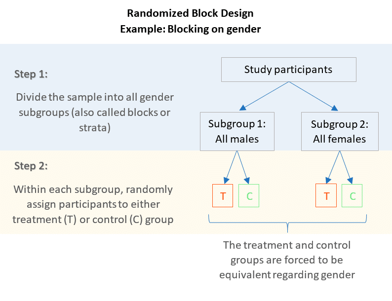
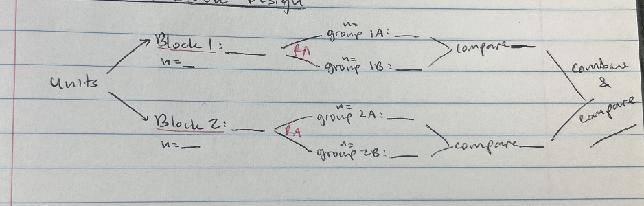
• Randomized Block Design: Groups similar subjects together and randomly assigns treatments to each group: 

  • Blocking is a technique that can control the response variable in an experiment

    

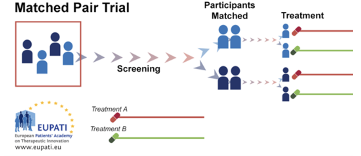
• Matched Pairs Design: one in which each subject is matched with another subject with similar variables. One of the paired subjects is randomly assigned to one study group, while the other is then assigned to the other study group.

  

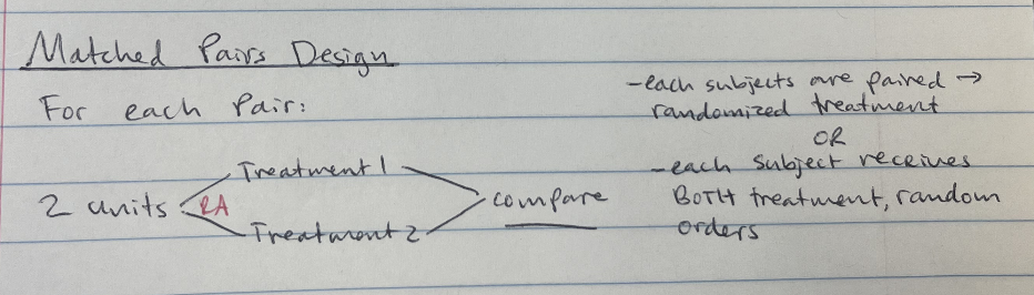
Details: Random assignment of subjects to treatment groups DOES NOT eliminate bias in response variable.

Variables: 🤗 💖

• Explanatory Variable: the variable that is used to explain or predict changes in another variable

• Response Variable: the variable that is being measured or observed to determine the effect of another variable

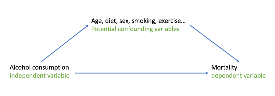
• Confounding Variable: related to the explanatory & effects the response

  • two variables are confounded if their effects on response variable cannot be distinguished.

    • ex.

      

Unit 5:

Probability = Longrun relative frequency

• Always between 0 and 1 (inclusive)

• Short-run

  • Unpredictable

• Long-run

  • Predictable

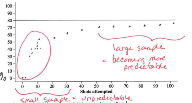
The Law of Large Numbers

• Law of large numbers - states that when an experiment is performed a large number of times, the relative frequency of an event tends to become closer to the true probability of the event;

  • that is, probability is long-run relative frequency. There is a sense of predictability about the long run.

• The law of large numbers has two conditions:

  • First, the chance event under consideration does not change from trial to trial.

  • Conclusions must be based on a very large number of observations.

• Example:

  • Flipping a coin, the more times you flip, the more its 0.5

Simulation:

• A technique for modeling random events in a way that matches real-world outcomes

  • Ex. roll die, toss coin, applet, RNG

• Evidence for a claim:

  • Assuming a claim is true, find the probability of getting the observed result or more extreme

    • less than 5% (<5%)

      • statistically significant

      • evidence against the claim

Sample Space

• Sample Space

  • The list of all possible outcomes

• P(E)= number of outcomes in E/total number outcomes in sample space

  • when each outcome is equally likely

Complement Rule

• P(A^c)= 1 - P(A)

  • Probability of an event NOT happening

• P(A and B) = P(A n B)

  • Both

• P(A or B) = P(A U B)

  • Either or both

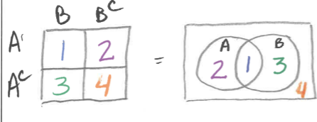
Two-way Table & Venn Diagram

Addition Rule

• P(A U B) = P(A) + P(B) - P(AnB)

  • P(A U B) = Union

  • P(AnB) = Intersection

• If events A and B are mutually exclusive (disjoint), they can’t occur together

  • P(A U B) = 0, so P(A U B) = P(A) + P(B

Conditional Probability

• The probability of one event given another event has occurred

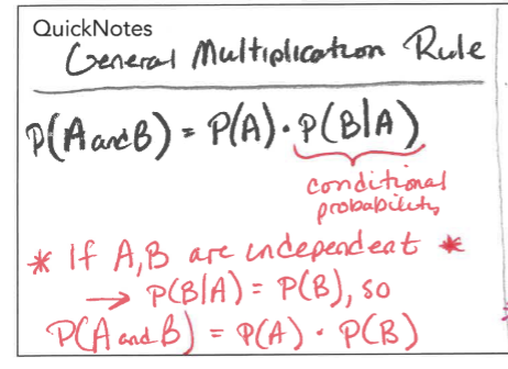
  • P(A/B) = P(A and B) / P(B)

Independent Events

• Knowing whether or not one event occurs does not change the probability of the other event

  • if P(A) = P(A/B) = P(A/B^c) then A and B are independent

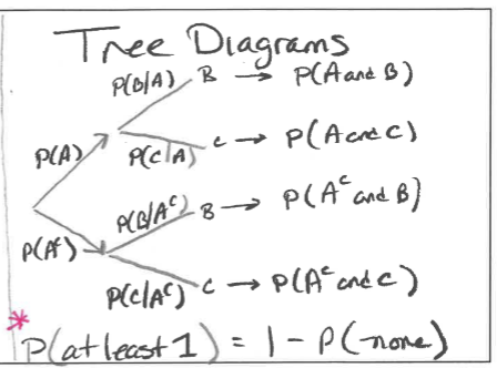
General Multiplication Rule

Tree Diagrams

Questions

Is percentile inclusive or exclusive, like do you count values below it or include that value

Evidence for a claim:

• Assuming a claim is true, find the probability of getting the observed result or more extreme

  • less than 5% (<5%)

    • statistically significant

    • evidence against the claim

• P(A U B) = Union

• P(AnB) = Intersection

#4 on test 2

#6 on test 3

#7 on test 3

#10 on test 3