Marginal rate and substitution

• MRSxy = oppurtunity cost, slope of indifference curve

A series of optimal consumer choices provides the theoretical basis for an individual demand curve

Diminishing marginal utility

• as we consume more of a good, the satisfaction we derive from 1 additional unit decreases

• rate of satisfaction diminishes with every 1 unit

• examples: food, cars

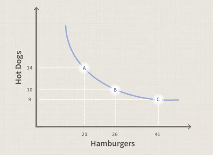
Indifference curves

• IC always has a negative slope if consumer likes both goods

• IC cannot intersect

• Every good can lie on one IC

• ICs are not thick

Demand Theory

• Substitute effect

  • Measures of consumer MRSxy, before and after the price change

  • Amount of additional food the consumer would buy to achieve the same level of utility (assuming a price decrease in one good)

  • Moving from one optimal curve to another

  • Steps:

    • Identify initial optimum basket of goods

    • Identify final optimum basket of goods, after the price change

    • Identify the decomposition optimum basket (DOB), attributed to the substitution effect

      • DOB must be on a BL that is parallel to BL2 following the price change

      • Assume that consumer retains same level of utility after the price change

• Income effect

  • Accounts for price change by holding the consumer’s purchasing power (following price change) constant and finding an optimum bundle on a new (higher/lower) utility function

    • Purchasing power - number of goods/services that can be purchased with a unit of currency (falls when price increases)

  • Measured from the DOB (B and Xb) to the final optimum bundle, following price change (C and Xc)

  • Both effects move in the same direction

• Law of Demand

  • At a higher price, consumers will demand a lower quantity of a good (vice versa)

  • Relates to diminishing marginal utility by compensating (off-set) DMU must be negatively related to quantity

  • Inverse relationship of price and quantity

  • Given the presence of diminishing marginal utility, in order to promote increased consumption, prices must fall

  • For a “normal good,” the increase in consumption results from a fall in price - this is driven by:

    • a lower MRSxy, while remaining on the same IC generates increased consumption of good X (substitute effect)

    • the theoretical increase in income necessary to lift the consumer to the higher IC, while keeping the ratio of prices at the new level (income effect)

  • Economic theory of demand always starts at the individual level. A horizontal summation of many individual demand curves provides a market demand curve. Market demand curves are always less steep than individual demand curves

Determinants of Demand

• Income

• Price of substitutes/complements

• Number of consumers

• Preference or tastes

  • These factors cause a market demand curve to shift (change in demand)

Individual Demand Curve

• a series of optimal choice bundles across different price levels (shown on price-quantity graphs)

Inferior Good

• whether the substitution effect or income effect dominates in an empirical not theoretical question

• Opposite of a normal good, demand falls when income rises

Non-price determinants of demand

• income (normal good)

• income (inferior good)

• preferences/tastes

• price of substitute/complement goods

• number of consumers

Perfect Competition

• Economic profit maximization is the assumed goal of private firms

  

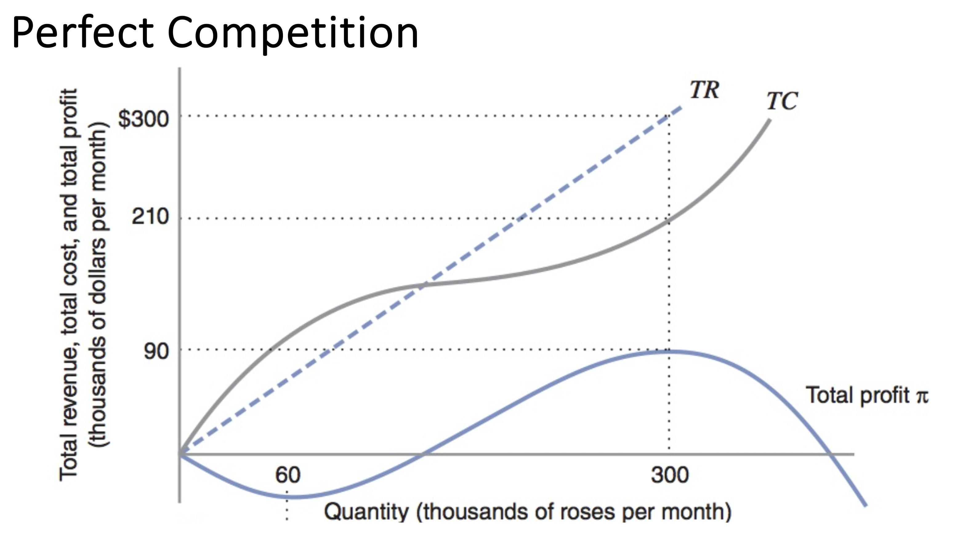
• Total cost represents the most efficient combination of inputs for a given level of output

• The rate at which total revenue (TR) changes with respect to change in output (Q) is marginal revenue (MR)

• MR = TR/Q = (Q*P)/Q = P

  

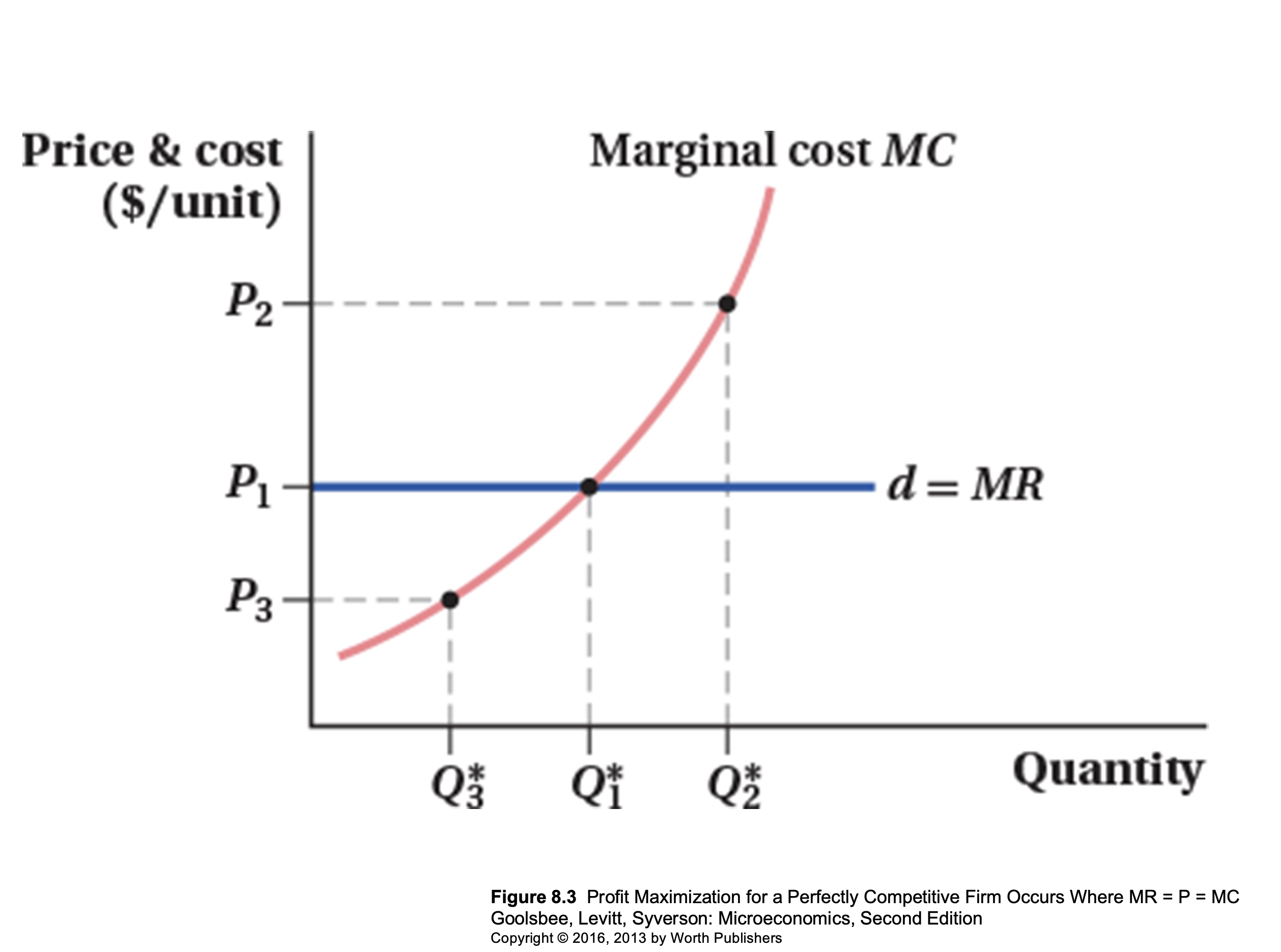
• Profits are maximized when marginal revenue = marginal cost

  • After the point where MR=MC, your profits will be negative

• Supply = MC, total cost optimized

Market Equilibrium

• the intersection of the demand and supply curves

• total cost is important as it is the basis of an individual firm’s supply curve

  • upward sloping section of the marginal cost curve is the supply curve

Efficiency of demand/supply curves

• Supply curves

  • Optimal combination of cost-minimizing inputs for each level of output

• Demand curves

  • Optimal combination of utility-maximizing goods for a given level of income

• Market supply curve

  • Horizontal summation of a series of individual supply curves

Supply Theory

• Supply - total amount of goods and services that producers are willing and able to purchase at a given price in a given time period

• Law of Supply

  • as the price of a product rises, the quantity supplied of the product will usually increase (ceteris paribus)

  • firms attempt to maximize product by increasing quantity supplied when the price is higher (and vice versa)

Non-price determinants of supply

• Changes in costs of factors of production

• Prices of related goods

• Indirect taxes and subsidies

• Future price expectations (producer)

• Changes in technology

• Number of firms

• Shocks

  • Markets only work when there is strong competition

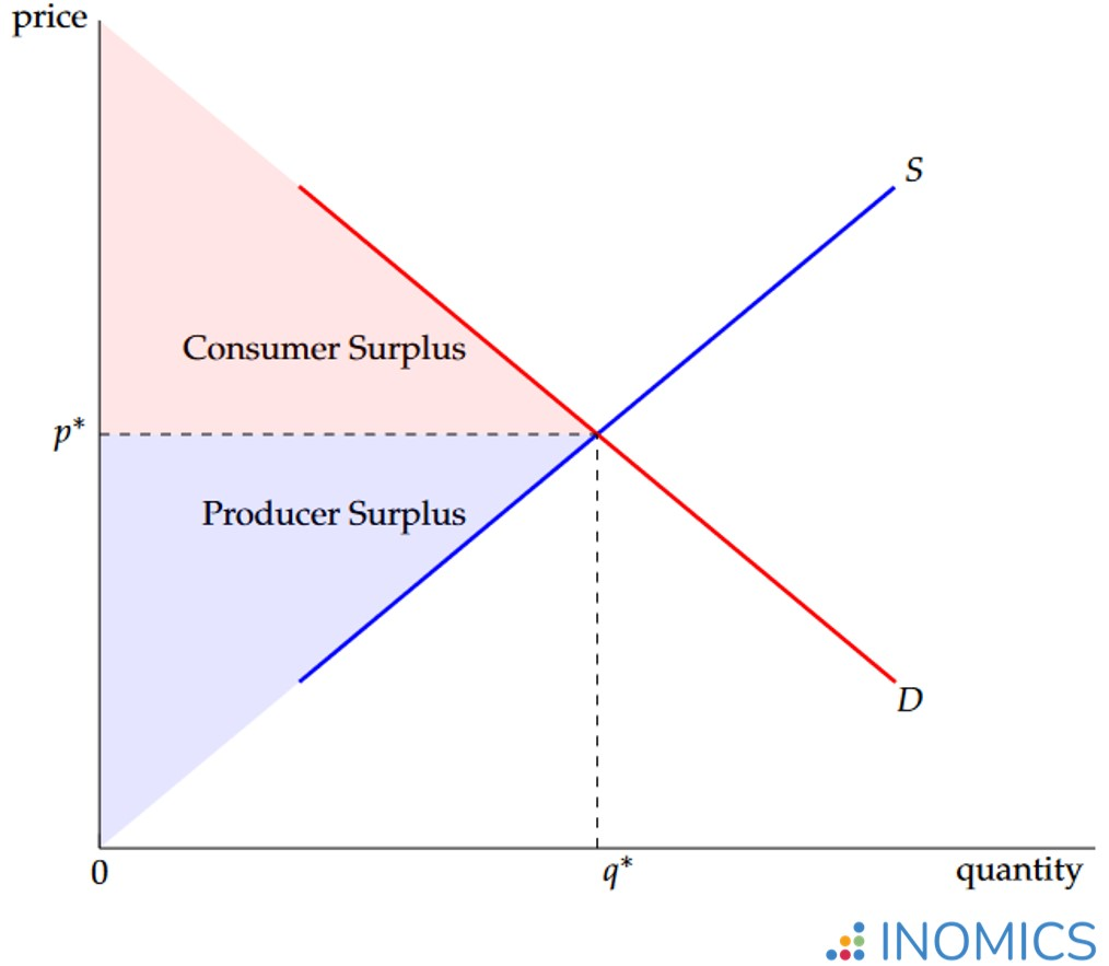
Market Equilibrium Graphs (supply + demand)

Consumer Surplus (C.S.) - willingness to pay and what they did pay

Producer Surplus (P.S.) - difference between market price and lowest price a producer uses to produce

Assumptions of perfectly competitive markets

• all actions (consumers/producers) have access and fully process all relevant information

• there are many small buyers and producers - all with equally negligible market power

• all actors are rationally self-interested

Welfare - theoretical surplus value left with different economic agents (consumers, firms, governments)

Production - market clearings

Optimal Allocation

• MR = MB (marginal benefit)

• Social surplus = consumer + producer surplus

• In a perfectly competitive market, social surplus is at its largest

• Analysis of surpluses are called “welfare analysis”

Price Mechanism Functions

A - allocation (resources are allocated to those who need it most)

R - rationing (not everyone in the market gets what they want, only those who have the same valuation of the product as the firms)

S - signaling (communication of information that drives other factors)

I - incentive (capitalist system is driven by incentives)

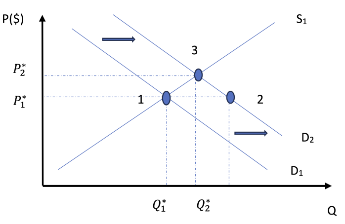
2 Demand Curves

2 Supply Curves

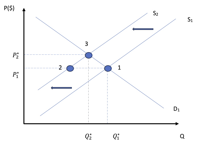
• Moving from point 1 to point 3 on both graphs

• Point 2 has excess supply/demand

• ARSI to move to the new equilibrium point

• At both equilibriums, there is optimal allocation

Structure of Microeconomics

• How do consumers and producers make choices in trying to meet their economic objectives?

  • Demand

  • Supply

  • Competitive market equilibrium

  • Elasticities of Demand

  • Elasticities of Supply

  • Critique of the maximizing behavior of consumers and producers

  • interaction between consumers and producers determine where resources are directed

  • welfare is maximized if allocative efficiency is achieved

  • constant change produces dynamic markets

  • consumer and producer choices are the outcome of complex decision making

• When are markets unable to satisfy important economic objectives - and does government interaction help?

  • Role of government in microeconomics

  • Market failure

    • externalities and common pool or common acess resources

    • public good

    • asymmetric information (imbalanced information held by consumers and/or consumers)

    • market power (single/small number of suppliers)

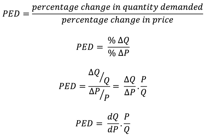
Price Elasticity of Demand (PED)

• measure of the responsiveness of the quantity demanded of a good subject to the change in price

  • Percentage change and differentiation to calculate

• PED = percentage change in quantity demanded / percentage change in price

  

• |PED| > 1 demand is relatively elastic

• |PED| < 1 demand is relatively inelastic

• |PED| = 0 demand is unitary

• PED = ∞ perfectly elastic

• PED = 0 perfectly inelastic

How can PED change along a straight line?

• as you move along the x-axis, it gets less elastic

  • as quantity increases, elasticity decreases

How does PED change across income levels?

• more elastic for lower income groups

• elasticity depends on the good (price-quantity relationship)

• quantity demanded changes, but not the demand curve

• “staples” are essential, less elastic

Determinants of Price Elasticity of Demand (PED)

• number of close substitutes; more subs = increased price sensitivity

• luxuries VS staples

• time - purchases made with longer time periods are generally more elastic

• proportion of income spent on the good

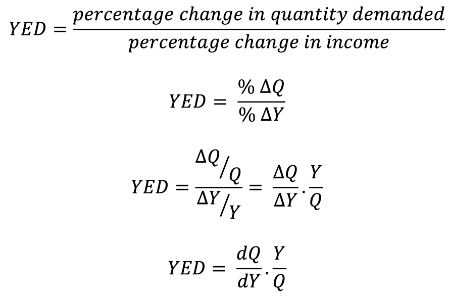
Income Elasticity of Demand (YED)

• measure of how much demand for a product changes when there is a change in the consumer’s income

• YED = percentage change in quantity demanded / percentage change in income

  

• YED to categorize inferior and normal goods

Engel Curve

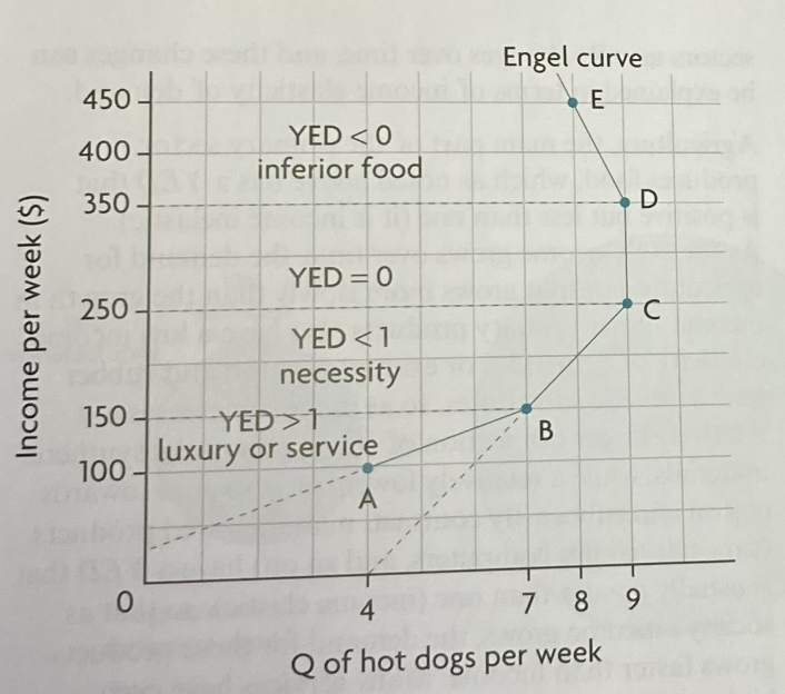
• axes → income and quantity

• YED > 1 luxury/service

• YED < 1 necessity

• YED > 0 normal good

• YED < 0 inferior good

• quantity demanded when income increases also increases then diminishes and goes backwards

• if you continue a segment AB with the same slope and that line cuts the y-axis, then it is a luxury

  • if it cuts the x-axis, it is a necessity

  • only works on income = y and quantity = x

Primary Commodities

• raw materials (cotton, coffee)

• inelastic demand (they are necessities)

• consumers are not everyday households, but manufacturers

Manufactured Goods

• made from primary commodities

• more elastic, as there are more substitutes

Why is YED important?

• For firms:

  • products with a high YED will see a demand increase when income increases (used to see maximum profit based off changes in income)

    • allocation of resources to fit income groups in products

    • if income falls, production of inferior goods increase because of YED rules

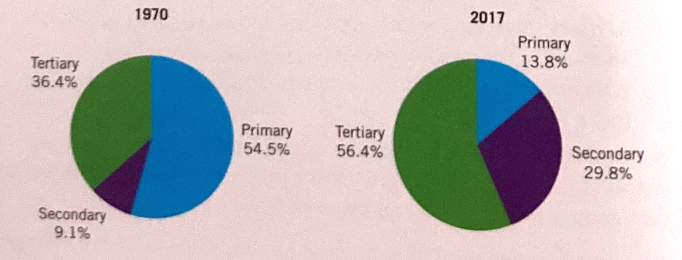
• Sectoral changes

  • primary sector: agriculture, fishing, extraction (forestry, mining)

  • secondary sector: manufacturing, takes primary products and uses them to manufacture producer goods (machinery, consumer goods) also includes construction

  • tertiary sector: service, produces services or intangible products (financial, education, information, technology)

  • shifts in the relative share of national output and employment

  • as countries grow and living standards improve, there is a change in proportion of the economy that is produced

  • extra income is spent on manufactured goods as the demand is more elastic than the primary products (using YED to measure/verify) ← same goes for the service sector

    

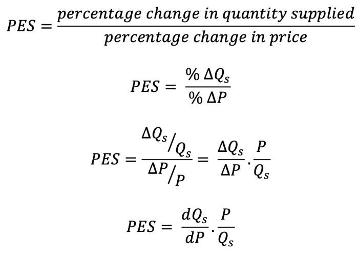
Price Elasticity of Supply (PES)

PES = percentage change in quantity supplied / percentage change in price

2.4 - Behavioural Economics

Assumptions of Rational Consumer Choice

• free markets are built on the assumptions of rational decision making

• in classical economic theory, rational means economics agents are able to consider the outcome of their choices and recognise the net benefits of each one

  • rational agents - will select the choice that reaps highest benefit/utility

• Rational choice theory - individuals use logic and sensible reasons to determine the correct choice (connected to an individual’s self-interest)

• Consumer Rationality

  • assumption that individuals use rational calculations to make choices which are within their own best interest (using all information available to them)

• Utility Maximization

  • economic agents select choices that maximize their utility to the highest level

• Perfect Information

  • information is easily accessible about all goods/services on the market

  • individuals have access to all information available at all times in order to make the best possible decision

Limitations of Assumptions of Rational Consumer Choice

• behavioural economics recognizes that human decision-making is influenced by cognitive biases, emotions, social, and other psychological factors that can lead to deviations from rational behaviour

• individuals are unlikely to always make rational decisions

• 5 limitations are shown below:

1. Biases

• biases influence how we process information when making decisions = influence the process of rational decision making

  • example: common sense, intuition, emotions, personal/social norms

• Types of Bias

  • Rule of Thumb - individuals make choices based on their default choice gained from experience (ex: same product from same company, but not the best possible choice)

  • Anchoring and Framing - individuals rely too heavily on an initial piece of information (anchor) when making subsequent judgements or decisions (ex: car dealer says car is worth $10,000 and you know it’s worth less, but this anchor of information causes you to purchase the car for a higher price)

  • Availability - individuals rely on immediate examples of information that come to mind easily when making judgements/decisions (causes individuals to overestimate the likelihood/importance of events/situations based on how readily available they are in their memory)

2. Bounded Rationality

• people make decisions without gathering all necessary information to make a rational decision within a given time period

• rational decision making is limited because of

  • thinking capacity

  • availability of information

  • lack of time available to gather information

• too many choices also cause people to make irrational decisions

  • example: in a supermarket, there are too many choices of products of the same good, making it difficult to reach a decision

3. Bounded Self-Control

• individuals have a limited capcity to regulate their behaviour and make decisions in the face of conflicting desires or impulses

  • self-control is not an unlimited resource

• because humans are influenced by family, friends, or social settings, it causes social norms to interfere in decision making (does not result in the maximization of consumer utility)

• decision making based on emotions → does not yield the best outcome

• businesses capitalize on the lack of bounded self-control of individuals when appealing to their target audience to maximize sales

4. Bounded Selfishness

• economics agents do not always act within their own self interest

• individuals do things for others without a direct reward

  • ex: altruism - selflessness without expecting anything in return

5. Imperfect Information

• information is not perfectly accessible due to:

  • intelluctual property rights

  • cost of accessing information

  • amount of information and options available

• people make decisions based on limited information

• asymmetric information may also lead to decisions based on limited information

  • when one party has more information than another

Choice Architecture

• intentional design of how choices are presented so as to influence decision making

• simplifies the decision making process

• 3 types, as shown below:

1. Default Choice

• individual is automatically signed up to a particular choice

• decision is already made even when no action has been taken

• individuals rarely change from the default change

2. Restricted Choice

• choices available to individuals are limited which helps individuals make more rational decisions

3. Mandated Choices

• requires individuals to make a specific decision or take a particular action by imposing a requirement or obligation

• mandated choices can be used to ensure compliance with regulations or societal norms, making it necessary for individuals to make certain decisions

Nudge Theory

• practice of influencing choices that economic agents make, using small prompts to influence their behaviour

• firms should use nudges in a responsible way to guide and influence decision making

• designed to guide people toward certain decisions or actions while still allowing them to have freedom of choice

• consumer nudges should be designed with transparancy, respect for individual autonomy, and clear societal benefits in mind

Profit Maximization

• most firms have the rational business objectiveof profit maximization

  • profits benefit shareholders as they receive dividends and also increase the underlying share price

    • an increase in the underlying share price increases the wealth of the shareholder

• profit maximization rule

  • when MC=MR, then no additional profit can be extracted from producing another unit of output

  • when MC<MR, additional profit can still be extracted by producing another unit of output

  • when MC>MR, the firm has gone beyond the profit maximization level of output and starts making a marginal loss on each unit produced (beyond MR=MC)

• in reality, firms find it difficult to produce at the profit maximization level of output

  • the level may be unknown

  • in the short term, they may not adjust their prices if the marginal cost changes

    • MC changes regularly and regular price changes would be disruptive

  • in the long-term, firms will seek to adjust prices to the profit maximization level of output

  • firms may be forced to change prices by the competition regulators in their country

    • profit maximization level of output often results in high prices for consumers

    • changing prices changes the marginal revenue

Growth

• increasing sales revenue/market share

• maximize revenue to increase output and benefit from economies of scale

  • a growing firms is less likely to fail

1. Revenue Maximization as a Sign of Growth

• in the short-term, firms may use this strategy to eliminate the competition as the price is lower than when focusing on profit maximization

• firms produce up to the level of output where MR=0

  • when MR>0, producing another unit of output will increase total revenue

2. Market Share as a Sign of Growth

• sales maximzation which further lowers prices and has the potential to increase market share

  • occurs at the level of output where AC=AR (normal profit/breakeven)

• firms may use this strategy to clear stock during a sale to increase market share

  • firms sell remaining stock without making a loss per unit

Satisficing

• pursuit of satisfactory/acceptable outcomes rather than profit maximization

  • decision-making approaach where businesses aim to meet a minimum threshold or standard of performance rather than striving for the absolute best outcome

• small firms may satisfice around the desires of the business owner

• many large firms often end up satisficing as a result of the principal agent problem

  • when one group (the agent) makes decisions on behalf of another group (the Principal), often placing their priorities above the Principal’s

Corporate Social Responsibility (CSR)

• conducting business activity in an ethical way and balancing the interests of shareholders with those of the wider community

• extra costs are involved in operating in a socially responsible way and these costs must be passed on to consumers

2.7 - Government Intervention

Why do governments intervene in markets?

• Influence (increase/decrease) household consumption

• provide support to firms

• earn revenue

• influence the level of production of firms

• provide support to low-income households

• correct market failure

• promote equity

Microeconomic forms of government intervention

• price controls

• indirect taxes

• subsidies

• direct provision of services

• command and control regulation and legislation

• consumer nudges

Price controls

• price ceiling + price floor

• Price Ceiling

  • maximum price

  • below equilibrium point

  • the point where the price ceiling is set is Pmax

    • at Pmax, firms are willing to supply Qmax but the consumers demand a quantity above Q*

  • 

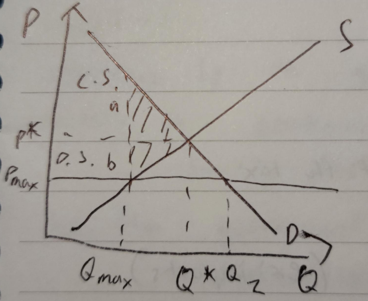
    • shaded area - 2 triangles, a and b

      • a = amount by which consumer surplus is reduced

      • b = amount by which produer surplus is reduced

  • excess demand shown by the values Qmax - Q1

    • managed through subsidies and tax breaks → costs

• Price Floor

  • minimum price

  • above equilibrium point (Pmin)

  • common in agriculture

  • 

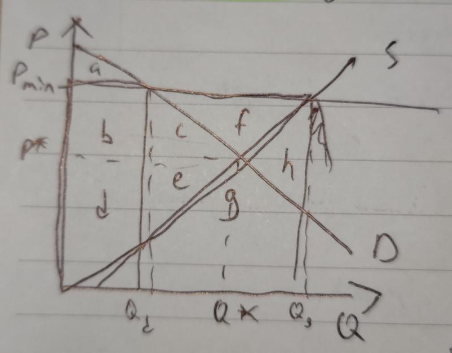
    • areas c, e, f, g, h are government expenditure → excess supply

  • producer surplus is increased (d+e → b, c, d, e, f)

    • f = directly from the government to the producers

  • a price floor creates welfare loss, indicating allocative inefficiency due to an overallocation of resources to the production of goods

  • society is getting too much of the good

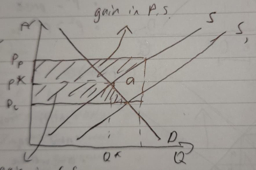
Indirect taxes

• imposed on spending to buy goods and services

  • both consumers and producers pay a share of the tax

  • firms practically pay the tax

• excise taxes - imposed on particular goods/services (ex: imports)

• taxes on spending - value added tax (VAT) or goods/services tax (GST)

• direct taxes are those directly paid to the government by taxpayers

• an indirect tax creates a tax wedge

  • consumers face a higher price, while producers receive a lower price

• 

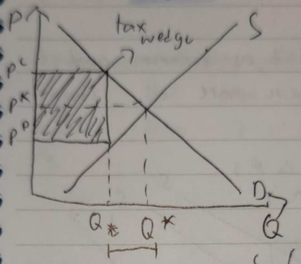
  • Qt - Q* → lost sales (potential sales but they are lost/didn’t happen because of the tax)

  • Pp - price for producers, marginal cost

  • area of rectangle = government revenue

  • Pc - price for consumers

  • Pc>Pp, so demand decreases

• 

  • shifts from S → S1

  • new equilibrium point formed at (Qt, Pc)

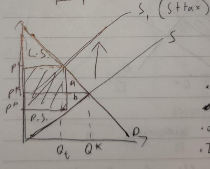
  • 2 triangles, a and b

    • a + b - welfare loss, Dead Weight Loss (DWL)

      • both disappear, allocative inefficiency

      • a - consumer surplus loss

      • b - producer surplus loss

  • 2 prices, C.S. and P.S. at different equilibriums

Subsidies

• assistance by the government to individuals (firms, consumers, industries)

• results in greater consumer and producer surplus

  • society loss as government spending on subsidy

• loss from government spending is greater than the gain in surplus

  • welfare loss (allocative inefficiency) due to overallocation of resources to the production of goods (overproduction)

• 

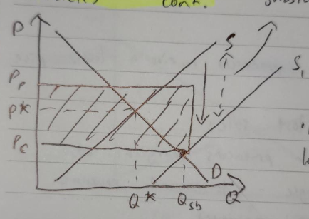
  • Pp and Pc switched (from indirect taxes), as consumers pay less and producers receive more

• 

  • a = dead weight loss (DWL) due to overproduction

  • supply curve shifts (S → S1) because of one of the non-price determinants of supply (subsidies)

    • S1 = S + subsidy

2.8 - Market Failures

• externalities are market failures, both positive and negative

Positive externality of consumption

• goods that when consumed, both the consumer and third parties benefit from it (ex: healthcare)

• 

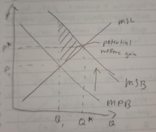
  • MSC - marginal social cost

  • MPB - marginal private benefit

  • MSB - marginal social benefit

  • in a free market, people would consume where MPB=MSC (Q1, P1)

  • (Q*, P*) where MSB=MSC is the socially optimal level (potential welfare gain) because from Q1-Q*, MSB>MSC

  • if MPB shifts from Q1-Q* (toward MSB), then the welfare loss is gained (potential welfare gain = welfare loss)

• underallocation of resources to this market (underproduction)

Merit Goods

• goods that are beneficial to consumers but people do not consume enough

  • people underestimate/ignore potential benefits, caused by imperfect access to information

• causes the demand to be lower than it should be

• examples: healthcare, education

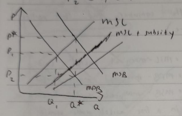
Government “fix”to positive externality of consumption

• subsidies/direct provision

  • shifts the MSC curve downwards

  • new socially efficient level at Q* but at a lower price (P2)

  • P2 < P1 < P*

  • 

• improving information (merit goods)

• legislation: government passing laws that force citizens to consume the good

Positive externality of production

• production of a good creates external benefits for third parties

  • ex: human capital: training employees

• 

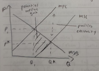
  • MPC - marginal private cost

  • produces where MPC=MSB, where Q1 is located (Q1 < Q*)

  • if production increases to Q*, there is a welfare gain (welfare loss turned into welfare gain)

• underallocation of resources → market failure, allocative inefficiency

Government “fix” to positive externality of production

• subsidies

  • causes MPC to be shifted downwards

  • full subsidy causes MPC=MSC when shifted

• direct provision

  • high cost

  • offering training through the state for firms causes MPC=MSC

Negative externality of consumption

• consumption causes adverse effects to third parties

  • ex: second hand smoking

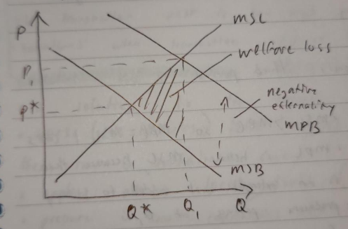• in a free market, people maximize their private utility so they consume at MPB=MSC

  • there is a welfare loss as MSC>MSB from Q*-Q1

  • overconsumption of goods

  • too many resources allocated

Demerit Goods

• goods that are harmful to the consumer but people still consume either because they are unaware of or ignore the potential harm

  • caused by imperfect information

  • demand is higher than it should be

  • creates negative externalities when consumed

• example: cigarettes

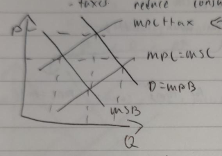
Government “fix” to negative externality of consumption

• indirect taxes

  • taxes reduce consumption

  • 

• legislation/regulation

  • making laws against the overconsumption of demerit goods

• education/raising awareness

Negative externality of production

• production of a good negatively impacts third parties

  • example: fumes from a factory

• 

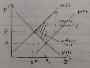
  • MSC<MPC so MPC=MSC+costs

  • MPC is below MSC, because there is an external cost added to society

  • producers produce at Q1

  • from Q1-Q*, MSC>MSB

  • welfare loss → market failure

Common Pool Resources

• rivalrous and non-excludable (linked to negative externalities)

  • rivalrous: if one person uses, others cannot at the same level of utility

  • non-excluable: very difficult to exclude people/groups of people from using

• typically natural resources

  • examples: fishing grounds, forests, atmosphere, etc.

Government “fix” to negative externality of production

• international agreements

• tradable permits

• carbon taxes

• legislations/regulations

• subsidies

Consequences for Stakeholders

• Ronald Coase → transaction costs are a way of attempting to measure the impossible, to measure the charges for externalities

• externality = transaction cost; there is a threshold where the transaction cost is too high so it is considered an externality

• sometimes when transaction cost is low, government intervention is not needed

Collective self-governance

• a solution to the over-use of common pool resources

• users take control of the resource and use them in a sustainable way

• applies at a local level (small communities)

• pressure in small communities to operate within social norms

• Ostom’s theories → no authority needed

Carbon Tax VS Tradable Permits

• carbon taxes are easier than tradable permits (design + implementation)

• carbon taxes are more difficult to manipulate for/against certain groups

• carbon taxes do not require as much monitoring

• carbon taxes are regressive

  • affects low-income groups more than high-income groups

• tradable permits more easily control the level of carbon reduction

• carbon taxes are easier to predict

  • businesses need certainty to plan for the future

Common Pool Resource - rivalrous and non-excludable

Private Good - rivalrous and excludable

Public Good - non-rivalrous and non-excludable (free-rider problem)

Quasi-public Good - non-rivalrous and excludable

Asymmetric information

• when one party has more information than the other

• buyers and sellers do not have equal access to information

  • either the buyer or seller has more information

Adverse Selection

• when one party in a transaction has more information on the quality of the good than the other party

Moral Hazard

• one party takes risks but does not face the full costs of these risks because the full costs of the risks are borne by another party

Perfect Competition / Rational Producer Behaviour

1. Suppliers and consumers are made up of equally small individuals

2. No barriers to market entry or exit

3. Firms are profit maximizing

4. Consumers are fully rational and consistent

5. Products sold are homogenous

6. Full information throughout the market

• cannot set the price:

  • 

Imperfect competition - monopolies

• monopoly market - where only one supply operates

  • the assumption of many small suppliers does not hold

  • 1 supplier with absolute control over the market price

• monopolist sets price at maximum total revenue

• as quantity increases, total cost increases, total revenue increases then decreases

Monopoly

• single seller facing many buyers

  • profit maximization condition: ΔTR(Q)/ΔQ= ΔTC(Q)/ΔQ

  • MR(Q) = MC(Q)

• MR>MC → firm increases Q

• MC<MC → firm decreases Q

• MR=MC → maximizes profit, cannot increase

• 

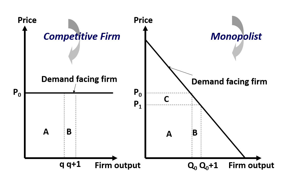
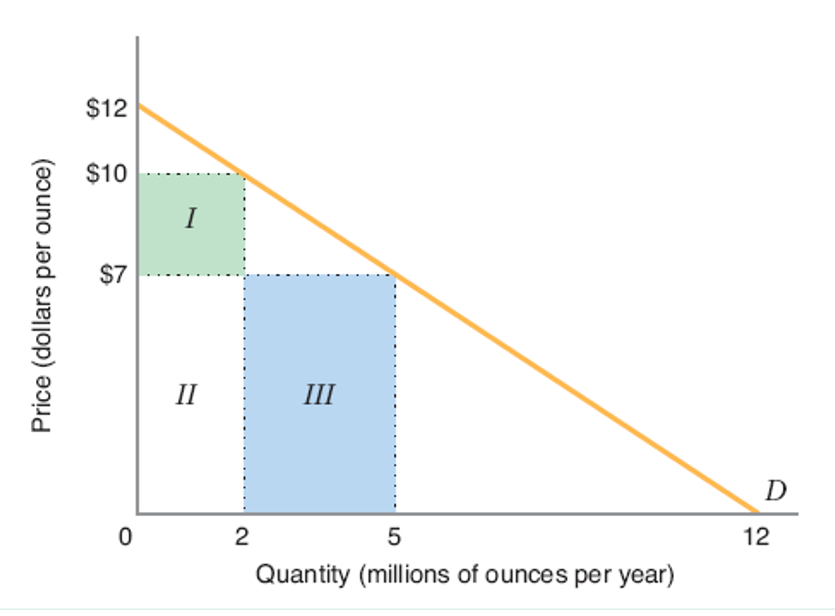
  • to sell more units, a monopolist lowers price

  • increase in profit = III while revenue sacrificed = I

  • change in TR = III-I

  • Area III = P * ΔQ

  • Area I = -Q * Δ

  • change in monopolist profit: P(ΔQ) + Q(ΔP)

  • MR = ΔTR/ΔQ = (PΔQ + QΔP)/ΔQ = P+Q(ΔP/ΔQ)

    • MR → P=increase in revenue due to higher volume - marginal units = Q(ΔP/ΔQ): decrease in revenue due to reduced price

  • AR = TR/Q = PQ/Q = P

  • price a monopolist can change to sell quantity Q is determined by the market demand curve (the AR curve = market demand curve)

    • AR(Q) = P(Q)

  • if Q>0, MR<P and MR<AC (MR lies below demand curve)

  • firms produce at MR=MC to maximize profits

• 

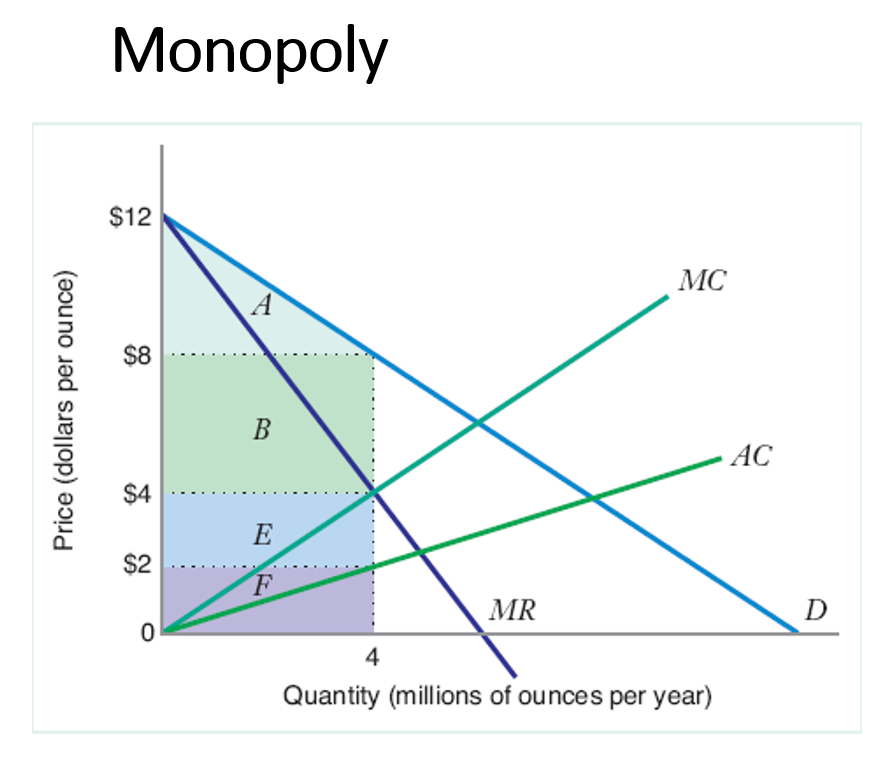
  • TR = B+E+F

  • Profit = B + E

  • L.S. = A

  • PED impacts the revenue

    • inelastic = more revenue

  • margin drives the average

• P=a-bQ TR=P*Q
  TR=(a-bQ)Q=aQ-bQ²
  dTR/dQ = a-2bQ

• Characteristics of a monopoly market

  • single firm in the market

  • no close substitutes - monopolist’s good or service is unique

  • high barriers to entry

• Long Run - factors of production are constant

• Short Run - only labour can change (not land or capital)

• Economies of Scale

  • 

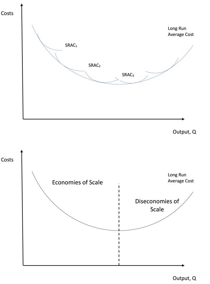
    • LRAC = Long Run Average Cost

    • considered a barrier to entry

    • as the monopolist increases production, their costs go down as output goes up

    • if new firms try to compete, they are unable to keep up with the costs of the large firm

Profits

• normal (π=0) → 0 profit

  • entrepreneurship is factored into the costs, so the wages are added into TC

• abnormal (π>0)

• loss (π<0)

• π = TR-TC = (PQ) - (CQ)
  π/Q = AR-AC = PQ/Q - CQ/Q = P-C
  AR = P, AC = C

  • normal profits are defined by the minimum revenue a firm must make to keep the business from shutting down (covers implicit and explicit costs)

• in a perfectly competitive market:

  • there are no profits in the long run

    • due to free entry + full information

    • there are economic profits in the short run

  • P*=AR=MR, all horizontal lines

• in a monopoly market:

  • can change the price but are still bounded by the demand, so AR and MR are no longer horizontal lines as they are in perfectly competitive markets

Perfectly Competitive Profits

• 

  • for a single firm

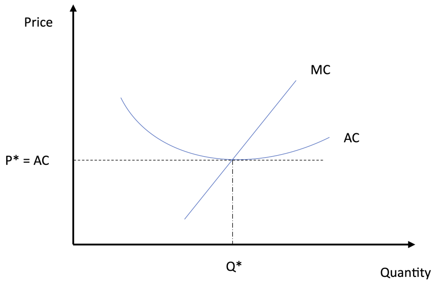
  • normal profits (P*=AC)

  • MC cuts AC at its minimum

  • P* = AR = AC (when AR=AC, π=0)

• 

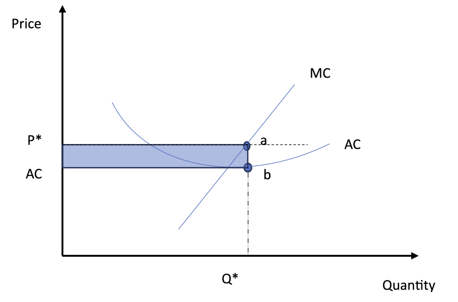
  • abnormal profits (P*>AC)

  • AR>AC, so profits are positive (π>0)

  • sells at Q*

  • shaded area = profit

• 

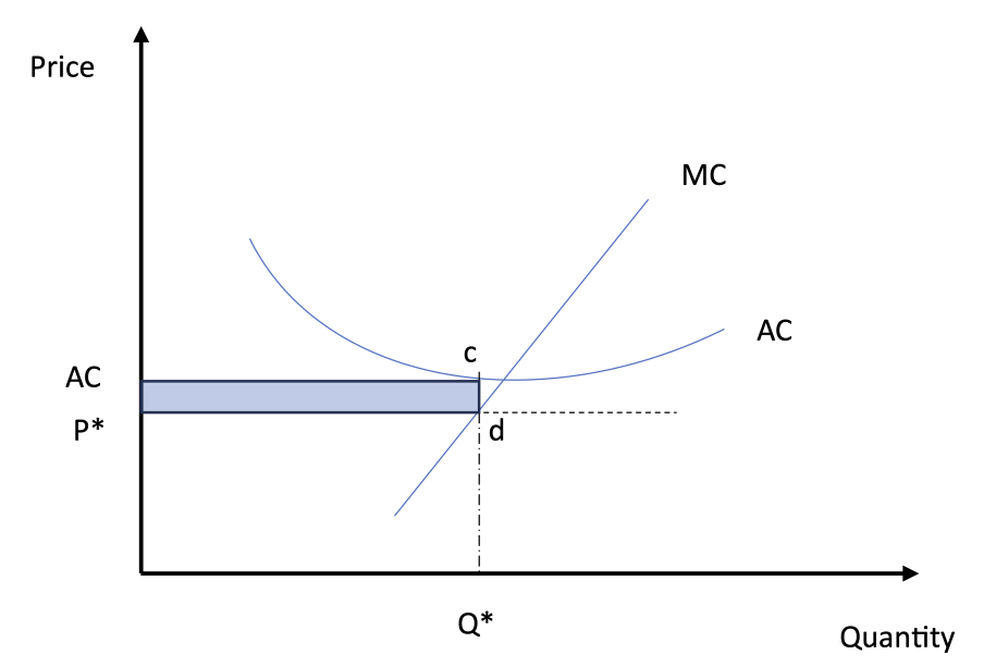
  • loss (P*<AC)

  • AR<AC, so profits are negative (π<0), so there is a loss

  • shaded area = loss

• Rules for a single firm in a perfectly competitive market

  • cannot determine price, so they determine the quantity at MR=MC due to the profit maximizing rule

  • they also determine profit when AR=AC (AR=AC=π=0)

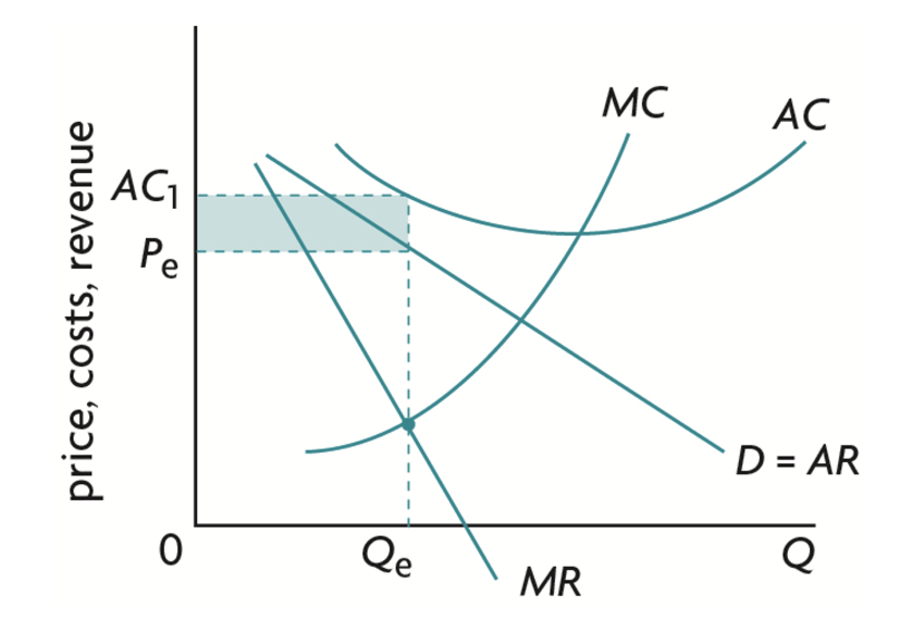
Monopolist Profits

• 

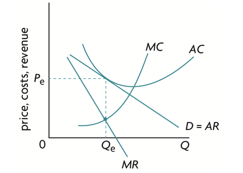
  • normal profit (π=0)

  • higher price, lower quantity

  • profit = difference between AR and AC

  • Q*=P*=AR=AC, so there is no

• Am

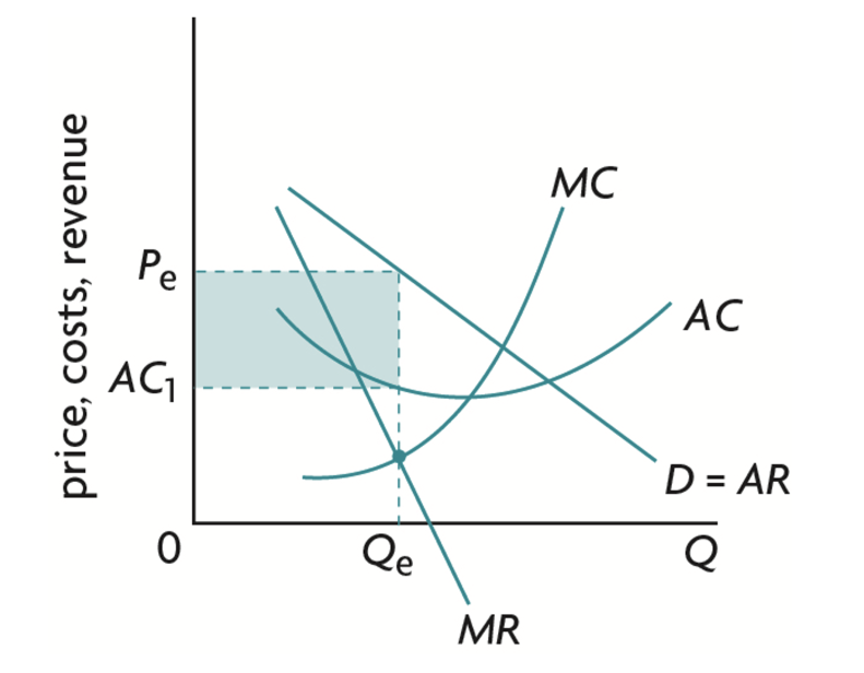
  • abnormal profit (π>0)

  • AR>AC

  • shaded area = profit

  • Q* determined where MR=MC, then find AR/D when it is equal to Q*

  • AC1 determined where AC is when it is at Q*

• 

  • loss (π<0)

  • same as abnormal profit, Q*, MR=MC, but AC>AR

  • shaded area = negative profit = loss because cost > revenue