DASC 120 Week 3 Lecture Ch. 5.2, 5.3
Confidence Intervals
Confidence intervals are ranges that encompass where we believe the "true” value of the population mean resides.
We determine a "Confidence Level" associated with how much risk we are willing to take that we have "got it wrong": an (alpha) level of 0.05 means that we are wi ing to take a 5% chance of getting a false positive. The corresponding "Confidence Level" to this is 95%
"We are 95% sure that the mean lies in this range”
A confidence interval estimates a population mean based on a sample.
Sometimes the point estimate is not as helpful as we'd like. To check the plausibility of our point estimate, we can create confidence intervals around that point.
A confidence interval gives us a range of values describing where we expect that point estimate to fall, given the potential for error in our calculations.
For instance, if we calculate a 95% confidence interval around the mean of our distribution, we are saying that we are 95% sure that the true value falls within the values in the range
“95% sure that the true value falls within the values in the range.”
CONFIDENCE INTERVALS - EXAMPLES
We take a poll of people and ask what they think the most fair price for an ice cream cone is. The mean of responses is $5.
But because of error, a more appropriate representation might be between 3 and 7 do ars. If s=1, then 3 and 7 are both 2 sd from the mean of 5, which is 95% of the distribution (assuming it is normal).
So we can say that we are 95% sure that the true value of the poll result is [3,7].
Confidence intervals give a range of plausible values for the true proportion
Confidence Intervals - Calculating
For Quantitative Data, the confidence interval at 95% may be calculated as
μ ± 2sd = 1.96 x n
For Qualitative Data, the confidence interval at 95% may be calculated as
phat ± 2sd = 1.96 × n
phat (proportion) ± standard error (proportion) = 1.96 × n
A 95% confidence level leaves 5% total in the two tails of the normal distribution.
Each tail has 2.5%, so you look for the z-value where the cumulative area = 0.975 (since 1 − 0.025 = 0.975).
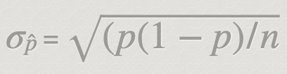
The standard error measures the variability of the sample proportion estimate
If we repeated a study 1,000 times and constructed a 95% confidence interval for each study, then approximately 950 of those confidence intervals would contain the true fraction of U.S. adults who suffer from chronic illnesses
A 90% confidence interval is narrower, not wider, because it uses a smaller critical value (z = 1.645) than the 99% interval (z = 2.58). Higher confidence requires a wider range.
Simply put, you are more sure of a wider range being true
Four Steps:
Prepare. Identify phat and n, determine CL
Check. Verify phat is nearly normal. For one-proportion CIs, use to check the success-failure condition.
Calculate: compute SE using phat, find z⋆, and construct CI
Conclude. Interpret CI in Context
Confidence Intervals - Confidence Level
What level should you use? — depends on industry!
For instance, we used 99.9% for diagnostic assays.
Pharma uses 99.99 or 99.999.
Logging? 85% might be fine!
Confidence Intervals - Checking Condition
Remember the Central Limit Theorem for proportions says that we must meet the following:
np ≥ 10
n(1 − p) ≥ 10
This means that both groups must be ≥ 10. We can use phat
Confidence Intervals - Standard Error
Find the standard error of the sampling distribution
Find the Z* for this sample —> if 95%, 1.96; if other, check z-table
(Remember, Z relates to standard deviations!)
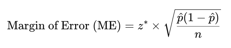
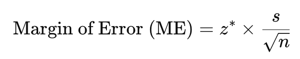
Margin of Error: Z* (σ of phat)
For proportions:
For means:
Confidence interval: ± 1.96 × n
Confidence Intervals - In Context
"In Context" means to describe the information in layperson's terms, casual conversational terms.
IE: CI=(2.4,4.5) at 95% related to the price of beans in Chicago:
We are 95% sure that the price of beans in Chicago is between $2.50 and $4.50