Economics HL 2.1-2.2 Microeconomics

Marginal rate of substitution

-MRSxy = oppurtunity cost, slope of indifference curve

a series of optimal consumer choices provides the theoretical basis for an individual demand curve

BL1 x I = Py1t x y1 + Px * x1

substituting one good for another based on preference

Diminishing marginal utility

• as we consume more of a good, the satisfaction we derive from 1 additional unit decreases

• rate of satisfaction diminishes with every 1 unit

Indifference curves (IC)

• IC always has a engative slope if consumer likes both goods on the axes

• IC cannot intersect

• Every good can only lie on one IC

• IC are not thick

Demand Theory

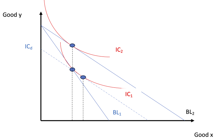
• Substitute effect - measures of consumer MRSxy, before and after Px

  • Amount of additional food the consumer would buy to achieve the same level of utility (assuming a price decrease in one good)

  • Moving from one optimal curve to another

  • Steps:

    • Identify initial optimum basket of goods

    • Identify final optimum basket of goods, after Px

    • Identify the decomposition optimum basket (DOB), attributed to the substitution effect

      • DOB must be on the BL that is parallel to BL2 following Px

      • Assume that consumer returns some level of utility after Px

• Income effect

  • Accounts for Px by holding the consumer’s purchasing power (following Px) constant and finding an optimum bundle on a new (higher/lower) utility function

    • Purchasing power - number of goods/services that can be measured from the DOB (B and XB) to the final optimum bundle, following Px (C and XC)

• Law of Demand

  • At a higher price, consumers will demand a lower quantity of a good (vice versa)

  • relates to diminishing marginal utility by compensating (off-set)

  • DMU must be negatively related to quantity

  • Inverse relationship between price and quantity

  • Given the presence of diminishing marginal utility, in order to promote increased consumption, prices must fall

  • For a “normal good” the increase in consumption - resulting from a fall in price - is driven by:

    • a lower MRSxy, while remaining on the same IC, generates increased consumption of good x (substitution effect)

    • The theoretical increase in income necessary to lift the consumer to the higher IC, while keeping the ratio of prices at the new level (income level)

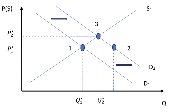
Determinants of Demand

• Income

• Price of substitutes / complements

• Number of consumers

• Preference of tastes

• These factors cause a market demand curve to shift ‘change in demand’

Individual Demand Curve

• a series of optimal choice bundles across different price levels (shown on price-quantity graphs)

Inferior good - whether the substitution or income effect dominates in an empirical not theoretical question

Economic theory for demand always starts at the individual level. A horizontal summation of many individual demand curves provides a market demand curve. Market demand curves are always less steep than individual demand curves

Non-price determinants of demand

• income (normal good)

• income (inferior good)

• preferences/tastes

• price of substitute/complement goods

• number of consumers

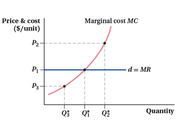
Perfect Competition

• economic profit maximization is the assumed goal of private firms

  

• Total cost represents the most efficient combination of inputs for a given level of output

• the rate at which total revenue (TC) changes with respect to change in output (Q) is marginal revenue (MR)

• MR = change in total revenue / change in quantity = price

• profits are maximized when marginal revenue = marginal cost

  • After the point where MR=MC, your profits will be negative

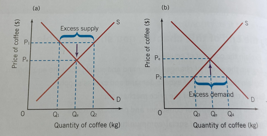
Market Equilibrium - the intersection of the demand and supply curves

Total cost is important as it is the basis of an individual firm’s supply curve

Upward sloping section of the marginal cost curve is the supply curve

Efficiency of demand/supply curves

• Supply curves

  • Optimal combination of cost-minimizing inputs for each level of output

• Demand curves

  • Optimal combinatinon of utility-maximizing goods for a given level of income

• Market supply curve

  • Horizontal summation of a series of individual supply curves

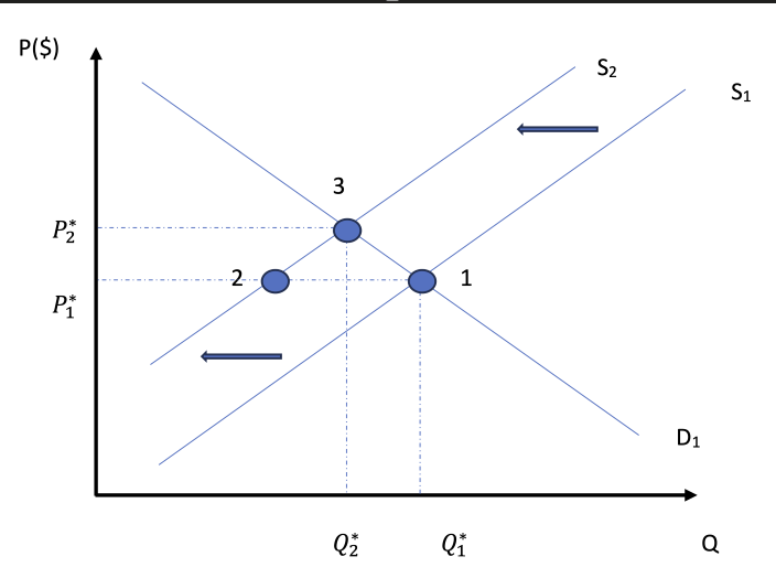
Non-price determinants of supply

• changes in costs of factors of production

• prices of related goods

• indirect taxes and subsidies

• future price expectations (products)

• changes in technology

• number of firms

• shocks

Markets only work when there is strong competition

Water-diamond paradox - why is water so cheap and diamonds so expernsive when water is more crucial? (marginal value) more utility is derived from water so price and utility are not correlated?

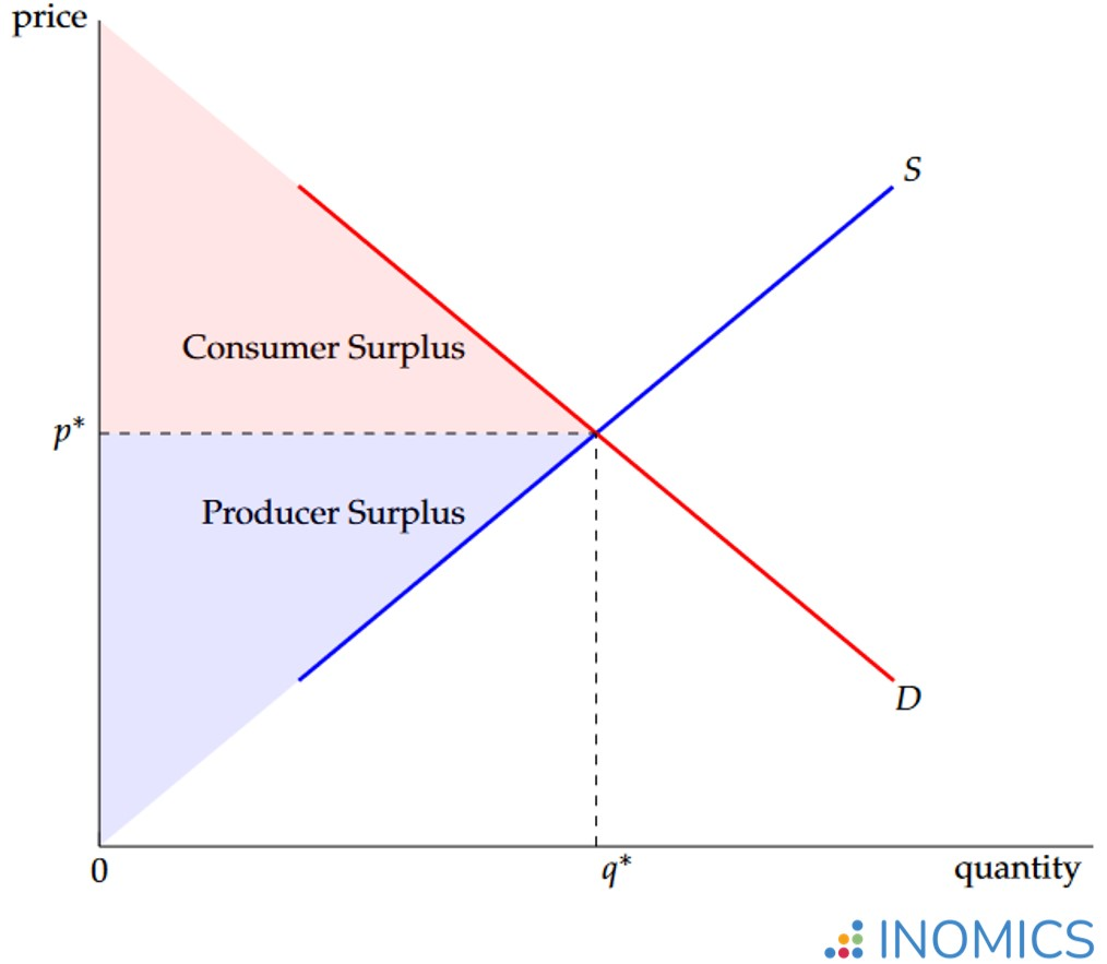
Consumer Surplus (C.S.) - willingness to pay and what they did pay

Producer Surplus (P.S.) - difference between market price and lowest price a producer uses to produce

Assumptions of perfectly competitive markets

• all actors (consumers/producers) have access and fully process all relevant information

• there are many small buyers and producers - all with equally negligible market power

• all actors are rationally self-interested

Total cost - cost-minimized, efficient with respect to the cost of production

Utility - utility maximized, efficiency with respect to generating well-being/satisfaction

Optimal allocation - perspective of society, not individual firms or consumears

Optimal choice bundles - any point on the demand curve, maximizing utility based off preferences and income

Welfare - theoretical surplus value left with different economic agents (consumers, firms, governments)

Production - market clearings

Optimal allocation

• MR = MB (marginal benefit)

• Social surplus = consumer + producer surplus

• In a perfectly competitive market, social surplus is at its largest

• Analysis of surpluses are called “welfare analysis”

Price mechanism functions

• Allocates (resources are allocated to those who need it most)

• Rationing (not everyone in the market gets what they want)

• Signals (communication of information that drives other factors)

• Incentive (capitalist system is driven by incentives)

• Some positive, some negative, some neutral

  

At both equilibriums, there is optimal allocation