Unit 3 P1

M16

• Aggregate Demand

  • all good and services (real GDP) that buyers are willing and able to purchase at different price levels

• Consumer spending has a large effect on the economy b/c it usually accounts for 2/3 of GDP

  • biggest impact on consumer spending is disposable income (income after taxes)

• Consumption functions show how a household consumer’s spending varies with the household’s current disposable income

• Marginal propensity to consume or MPC is the increase in consumer spending when disposable income rises by $1

• Consumption Function graph

  • y intercept, A, is the amount the household would spend if its current disposable income was 0

  • slope of the consumption function is the MPC

• Effects of Government Spending

  • If the government spends x amount of money, aggregate demand (AD) will not increase by the same amount

  • Government spending becomes income for consumers → AD increases

  • Consumers take that money and spend, further increasing AD

    • The amount by which AD increases depends on how much new income consumers save

      • if they save a lot, spending and AD will increase less and vice versa

• The Multiplier Effect

  • An initial change in spending will set off a spending chain that is magnified in the economy

  • Total change in GDP = Multiplier * Initial change in spending

  • Calculating the Spending Multiplier

    

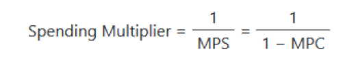
• Marginal Propensity to Save (MPS)

  • How much people save rather than consume when there is a change in income

• MPS = 1 - MPC (b/c people can either save or consume)

• Planned Investment Spending

  • decreases during economic downturns or periods of uncertainty

    • rising interest, lower consumer confidence, anticipated declines in demand

M17

• Inverse relationship between price level and Real GDP output

  • if price level increases (inflation) → real GDP demanded falls

  • if price level decreases (deflation), real GDP demanded increases

• Aggregate Demand (AD) Curve

  • Changes in price level don’t shift the curve, instead they cause a move along the curve

  • Why is AD curve downward sloping

    • Wealth Effect

    • Interest Rate Effect

    • Foreign Trade Effect

• Wealth effect

  • higher price levels reduce purchasing power of money → decreases quantity of expenditure

  • lower price levels increasing purchasing power → increase expenditures

  • Decrease in income taxes → increased expenditures

  • Expected increase in future income leads to increase in spending

• Interest Rate Effect

  • Price levels increase → lenders charge higher interest rates to get a return on their loans

  • Higher interest rates discourage consumer spending and business investment

  • As price level goes up, output goes down

• Foreign Trade Effect

  • U.S. price levels rise → foreign buyers purchase fewer U.S. goods and Americans buy more foreign goods

  • Exports fall + imports rise → real GDP demanded falls

  • Price level goes up → output goes down

• Shifters of Aggregate Demand

  • Increase in spending shifts AD right and vice versa

  • 1. Change in Consumer Spending

    • Higher incomes

    • consumer expectations

    • household in debt

    • taxes

  • 2. Change in Investment Spending

    • interest rates

    • future business expectations

    • productivity and technology

    • business taxes

  • 3. Change in Government Spending

    • Government expenditures (defense + public works)

  • 4. Change in Net Exports

    • exchange rates (currencies)

    • national income vs. abroad

M18 Aggregate Supply

• Aggregate Supply (AS)

  • amount of goods and services (real GDP) that firms will produce in an economy at different price levels

  • differentiates btwn short run and long-run and has two different curves

• Short Run AS

  • wage and resource prices will NOT increase as price levels increase

• Long Run AS

  • wages and resources prices will increase as price levels increase

  • In the short run, if total revenue increases, real profits will increase; however, in long-run AS workers will demand higher wages to match prices → nominal profits increase, but since all prices and costs have increased, REAL profits are unchnaged

  • If real profit doesn’t change the firm has no incentive to increase output

• Long Run (LR) Aggregate Supply (AS) graph

  • quantity in the long run is a fixed quantity, vertical line

  • assumption: in the long run, economy will be producing at full employment

• 3 Shifters of Aggregate Supply

  • Change in Resource Prices

    • prices of domestic and imported resources

    • supply shocks

    • inflationary expectations

      • i.e. if producers expect higher prices in the future ,workers will demand higher wages and costs will increase → decrease AS

  • Change in Actions of government (NOT GOV SPENDING)

    • taxes on producers

    • subsidies for domestic producers

    • change in productivity

  • change in productivity

• Increase in national production → curve shifts right and vice versa

M19

• Combination of AD and AS shows economy at full employment output

• inflationary and recessionary gaps

  • economy can either be at full employment, recessionary gap, inflationary gap

• inflationary gap

  • output is high and unemployment is less than NRU

  • actual GDP is above potential GDP (quantity is greater than LRAS)

  • correct by shifting SRAS to the left

• Recessionary gap

  • output is low and unemployment is greater than NRU

  • actual GDP is below potential GDP

  • can be corrected by shifting SRAS to the right

• Economic growth can only happen with an INCREASE in Ivestment Spending on Capital goods or capital spending

  • Capital Goods (CG) are things that companies purchase to increase their output in the future

  • Capital Spending (CS) includes things like machines, warehouses, new technologies etc.

  • Investment Spending actually causes a shift in both AD and AS

    • shift in AD caused by company’s increase in spending

    • shift in AS is caused by company’s new output as a result of the spending