Eco101: Lecture 11, Price Discrimination and Oligopoly

Page 1

Title & Introduction

• Economics 101 Lecture 11: Finer Points of Price Discrimination and Oligopoly

• Speaker: Loren Brandt, Department of Economics, University of Toronto

Page 2

Price Discrimination

• Definition: A business practice of selling identical goods at varying prices. → Selling the same good, difference price.

• Necessary Conditions:

  1. Market Power (not necessarily monopoly) → Setting its price

     2. Absence of Arbitrage, NONE → Seeing a product where prices are different, you want to buy LOW and sell HIGH.

     • Expect to happen to price in two markets: Price becomes the same which undermines price discrimination

  3. Capability to sort consumers based on willingness to pay (WTP) or elasticity

     • Identify who HWTP costumers are compared to the lower individuals.

• Types of Price Discrimination:

  1. Between Consumers: Different prices for different consumers.

  2. Within Consumers: An individual pays varying prices for different units purchased.

Page 3

Insight on Price Discrimination

• Price discrimination is generally the standard; single price monopolists are the irregular case.

Page 4

Differentiation Among Consumers

• Two Interpretations of Consumer Behavior:

  1. Each consumer may demand only one item based on high vs low WTP.

  2. Consumer or group demand displays elasticity, differentiating between inelastic (high WTP) and elastic (low WTP) demand.

• Objective:

  • Charge a higher price to consumers in the high WTP group and a lower price for the low WTP group.’

    Why:

Page 5

First-Degree Price Discrimination

• Assumption: Each consumer demands at most one unit.

• WTP Awareness: The seller is assumed to know each buyer’s WTP, effectively 'stamped on their forehead'.

• Optimal Pricing Strategy for Individual i:

  • Pi = max{WTPi, MCi}

• Graph: Illustration of price vs quantity with a marginal cost (MC) of 2.

Highest Willingness to pay

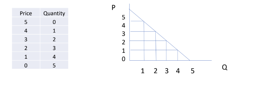
• 1st individual= 4

• 2nd individual= 3

• 3rd Individual= 2

• 4th Individual= 1

Why do they have an incentive to sell an additional unit: To sell more

Page 6

Implementation Problems of Price Discrimination

• Difficulty in determining WTP, as high WTP consumers lack incentive to disclose their WTP.

• Possible Solutions:

  1. Third-Degree Price Discrimination( Something observable that society can view and make assumptions) Group consumers who provide proof of belonging to a specific group for a lower price. International students vs domestic students.

  2. Second-Degree Price Discrimination: Allow consumers to self-select into groups by overcoming certain hurdles for discounts. Real Life examples, coupons: consumers can choose to use coupons to receive discounts on their purchases, effectively allowing them to self-select into a lower price tier based on their willingness to engage with promotional offers. Assumptions: Lower income, Lower WTP

Page 7

Third-Degree Price Discrimination

• Characteristics: Pricing is based on observable and non-modifiable traits.

• Correlation: The characteristic is linked to WTP (elasticity of demand).

• Pricing Strategy: Charge higher prices to groups with less elastic demand and lower prices to more elastic demand groups.

• Examples:

  • Dry cleaning, public transit pricing (TTC), subscription rates, pharmaceuticals (prices lower in Canada compared to the US).

Page 8

Demand for Microsoft Office

• Demand Curve Visualization: Total demand in millions of copies at various price points.

• Key Points:

  • At $75, all consumers including students will purchase.

  • At $225, only business owners will purchase.

  • At $150, both business owners and standard users are willing to buy.

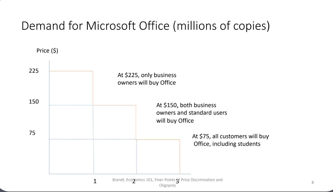
This illustrates the concept of price discrimination, where different prices are charged to different consumer groups based on their willingness to pay.

Page 9

Impact of Price Discrimination on Total Surplus

• Generally, total surplus increases with price discrimination; however, exceptions exist.

  • Example:

    • Without price discrimination, price to non-affiliated (PNA) = $100, with price discrimination: Price to US (PUS) = $110 and Canada (PC) = $90.

  • Net Effect: Gains in Canada must surpass losses in the US for total surplus to increase.

Page 10

Second-Degree Price Discrimination Logic

• Consumers receive lower prices upon overcoming hurdles:

  • Examples include clipping coupons, waiting in line, or traveling during off-peak hours.

  • Outcomes: Differentiation based upon willingness to jump hurdles, influencing price sensitivity and WTP.

Page 11

Second-Degree Price Discrimination – Consumer Sorting

• Offer different characteristic bundles or quantities to consumers:

  • High WTP (inelastic demand) individuals obtain premium bundles.

  • Low WTP (elastic demand) individuals choose less desirable products.

• Examples:

  • iPad storage options (1TB vs 256GB pricing) and book formats (hardcover, paperback, Kindle).

Page 12

Differentiation Between 2nd and 3rd Degree Price Discrimination

• Key Question: Is the lower price accessible to everyone?

  • Second Degree: Yes.

  • Third Degree: No.

Page 13

Within-Consumer Price Discrimination

• Assumes all consumers have identical marginal willingness to pay (MWTP) schedules.

• Discrimination Mechanism: Effectively charges different prices for each unit, similar to first-degree price discrimination.

• Example of Schedule: MWTP declining as quantity increases vs constant marginal cost.

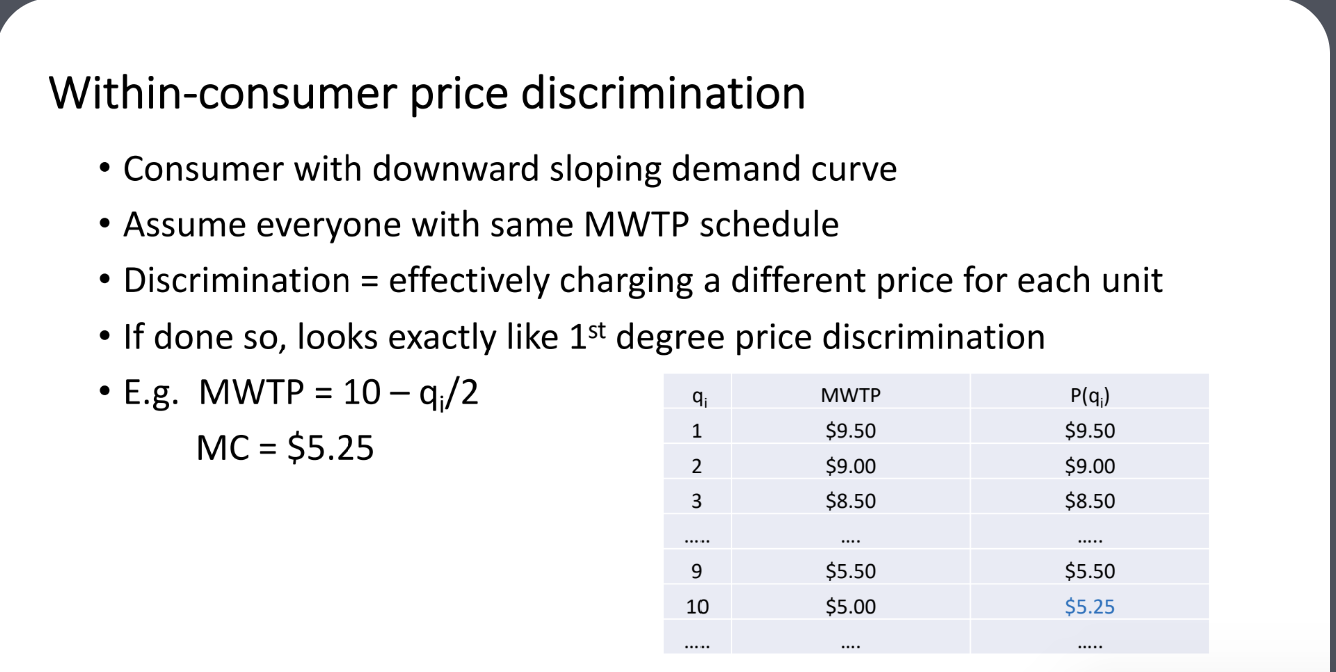
This approach allows firms to capture more consumer surplus by tailoring prices to individual consumer demand, thereby maximizing profits.

Page 14

Quantity Discounts

• Example Case: Ralph’s MWTP schedule illustrates the reaction to quantity discounts:

  • Pricing scheme allows for discounts based on purchase volumes (10% off for buying 2, 30% off for buying 3).

  • Optimal Strategy: Works effectively as long as firm’s marginal cost remains below specified threshold.

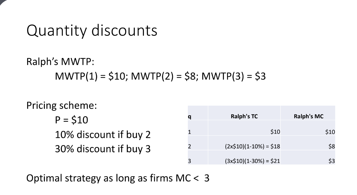
If he buys 2 units: Gets 10% discount, he pays $18, MC=$8

if buys three, gets 30% discount, cost is 21 and Mc is 3

How do we calculate MC is this example:

• To calculate the marginal cost (MC) in this example, we need to determine the change in total cost when an additional unit is produced or purchased. For instance, when the consumer increases their purchase from 2 to 3 units, the total cost changes from $18 to $21, resulting in a marginal cost of ( MC = \frac{\Delta TC}{\Delta Q} = \frac{21 - 18}{3 - 2} = 3. ) This shows that the marginal cost of producing the third unit is $3.

Page 15

Oligopoly and Game Theory

• Oligopoly Defined: A market structure characterized by a few firms supplying similar or identical goods.

Do I care what other firms do: No, because → other firms wont have affect on market price, doesn’t influence market outcome

• Key Features: Assumed barriers to entry, preventing other firms from entering (high fixed cost)

• Duopolist Scenario: Involves two firms.

• Strategic Setting: Payoffs depend on actions from other agents (firms).

• Game Theory: Analyzes decisions in strategic contexts, leading to outcomes like Nash Equilibrium.

• Analyzing how firms behave and making such predications

Nash Equilibrium→ A situation where neither firm has an incentive to deviate from their chosen strategy, given the strategy of the other firm.

Page 16

The Prisoner’s Dilemma

• Finding if a firm has a dominant strategy.

• Setup: Two criminals are questioned separately, and outcomes depend on individual strategy choices.

• Dominant Strategy: Each player wants to minimize their jail sentence, independently of other's choices.

• Tension Highlighted: Conflicts arise between collective good and individual benefit; equilibrium does not maximize group payoffs.

Page 17

Solving the Prisoner’s Dilemma

• Thelma's Decision Matrix: Outcomes based on Thelma and Louise's decision (confess vs remain silent) evidenced through potential years of imprisonment.

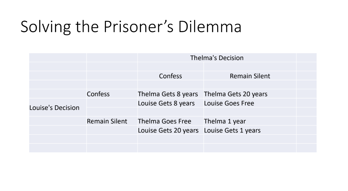
Lousies decisions. (Looking at Thelma’s decision)

• If Louise confess ( Look at Thelma confess) - 8 years

• If Louise is quiet (

• If both confess, they each serve 5 years.

• If one confesses while the other remains silent, the confessor goes free while the silent partner serves 10 years.

• If both remain silent, they each serve 1 year, demonstrating the tension between individual rationality and collective benefit.

Page 18

Dominant Strategy as Special Case of Nash Equilibrium (NE)

• NE Definition: A strategy profile where no player can achieve a higher payoff by changing their strategy while others remain constant.

• Alternative Definition: In a NE, each player's strategy is the best response to others' actions.

Page 19

Oligopoly: Multiple Strategic Settings

• Assumption Structure: Barriers to entry and standardized products.

• Cournot Assumptions:

  1. Firms choose quantities simultaneously.

  2. Market adjusts pricing to clear all units.

  3. Firms decide on capacity based on market expectations.

Page 20

Pricing in a Cournot Duopoly

• Price Function: Describes the relationship between market quantity and marginal willingness to pay (MWTP).

• Demand Analysis: Establishes the effect of one firm's quantity decision on the overall market.

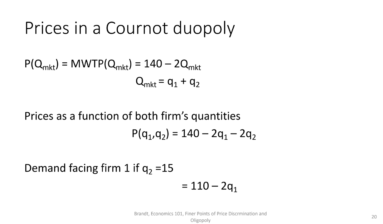
Implies: P

Page 21

Analyzing Cournot Outcomes -firms determines how much is produced.

• Demonstrates that split monopoly equilibrium cannot be a Nash Equilibrium during single period competition and thus reveals competitive outcomes land between monopoly and perfect competition in prolonged interactions.

• In models of cournot: As firms increases, level of output will be in between monopoly and perfect competition.

Why is it between monopoly and perfect competition:

Page 22

Solution Under Monopoly

• MR and MC Analysis: Establishes marginal revenue and cost for determining optimal production quantity.

• Profit Maximization: Refers to intersection point of MR and MC curve.

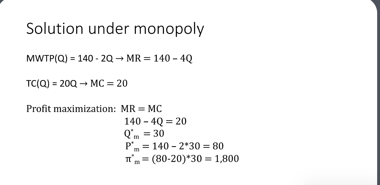
This point indicates the level of output where profits are maximized, as producing beyond this quantity would result in higher marginal costs than marginal revenue.

Page 23

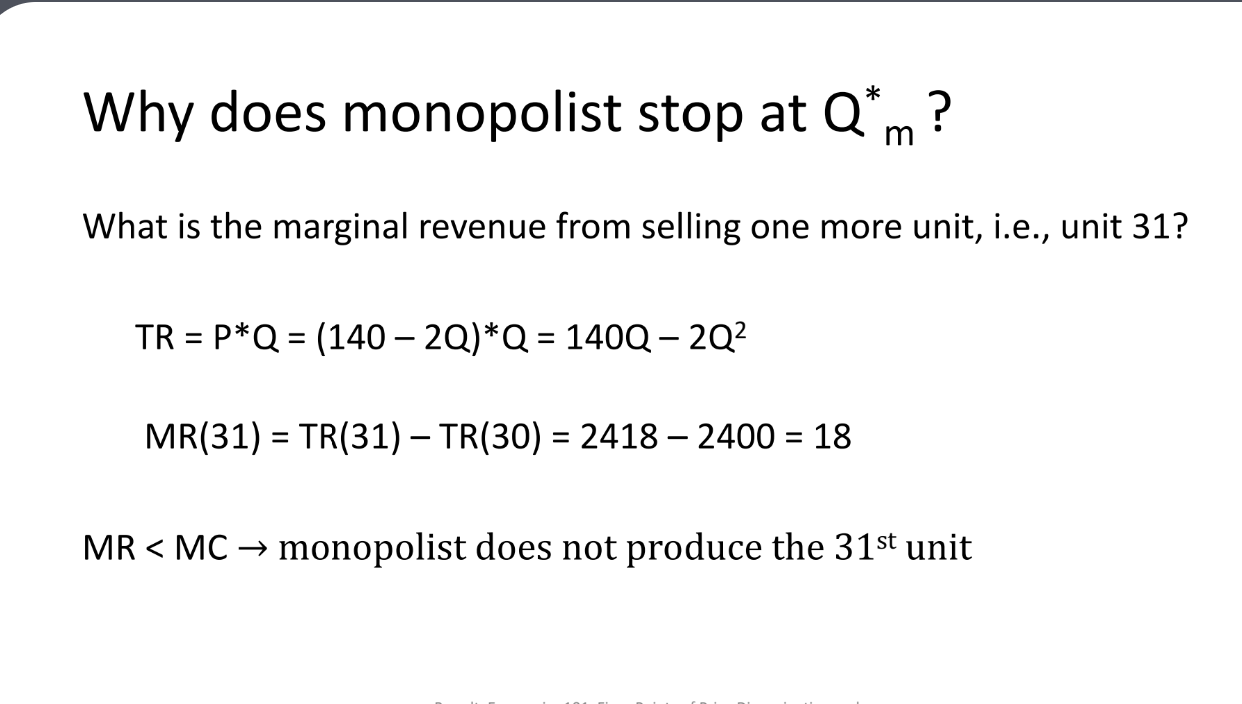
Monopolist Production Decisions

• Marginal Revenue Calculation: Evaluates additional revenue against the cost for producing the next unit of output.

• Optimal Production Decision: Determining production limits based on revenue falling below marginal cost.

• Price Discrimination: Selling the same product at different prices to different consumers, maximizing profits by capturing consumer surplus.

Why doesn’t it sell the 31st unit?: Because the marginal revenue generated from selling the 31st unit would be less than the marginal cost of production, leading to a decrease in overall profit.

• To do so: Lower the price. This strategy allows firms to increase sales volume and optimize their pricing structure, ultimately enhancing profitability in a competitive market.

Page 24

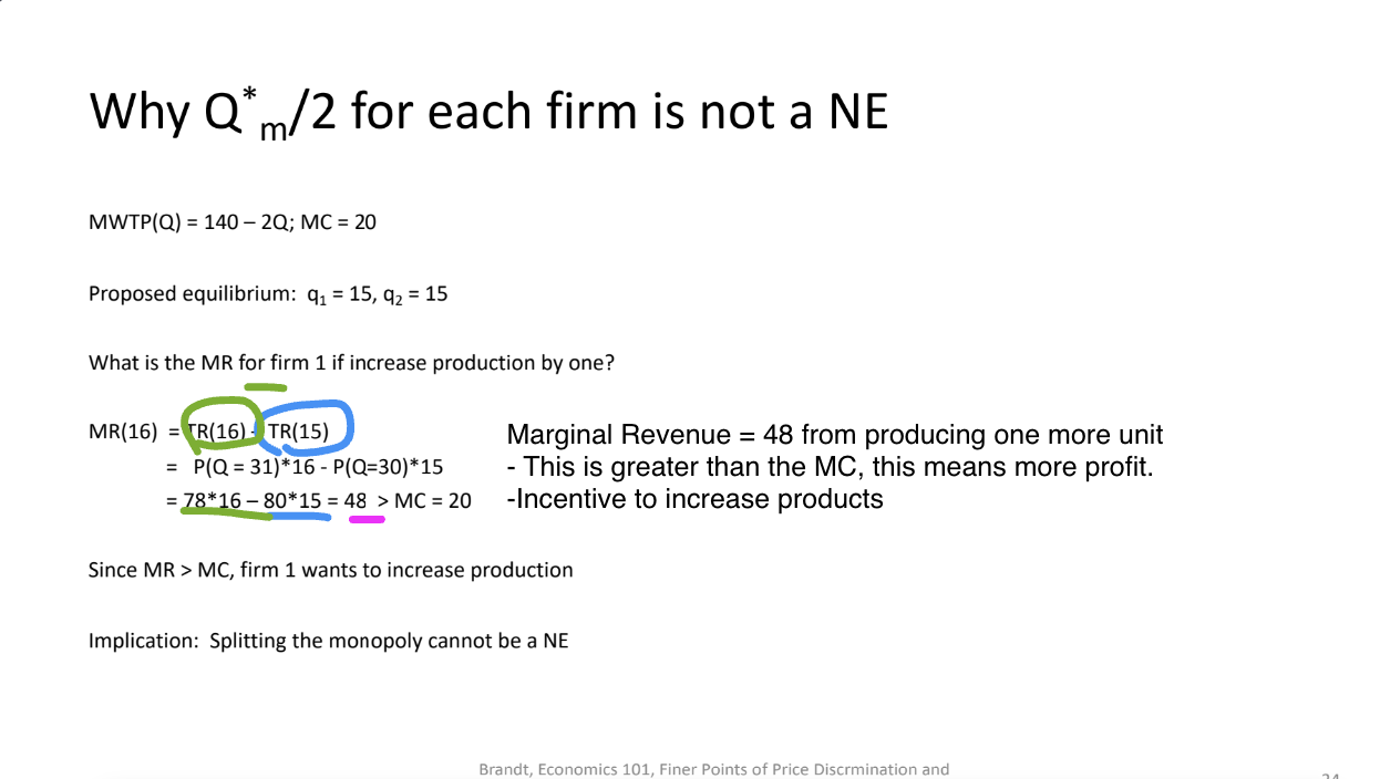
Why Q*m/2 for Each Firm is Not a Nash Equilibrium

• MR vs MC Analysis: Evaluates firm responses to production increases showcasing each firm's inclination to produce beyond the proposed equilibrium.

For the 16th unit: the marginal cost for Firm A is less than the marginal revenue, indicating that Firm A has an incentive to increase production to maximize profits, while Firm B will continue to operate at its current output level.

Originally: They are producing 15t

Page 25

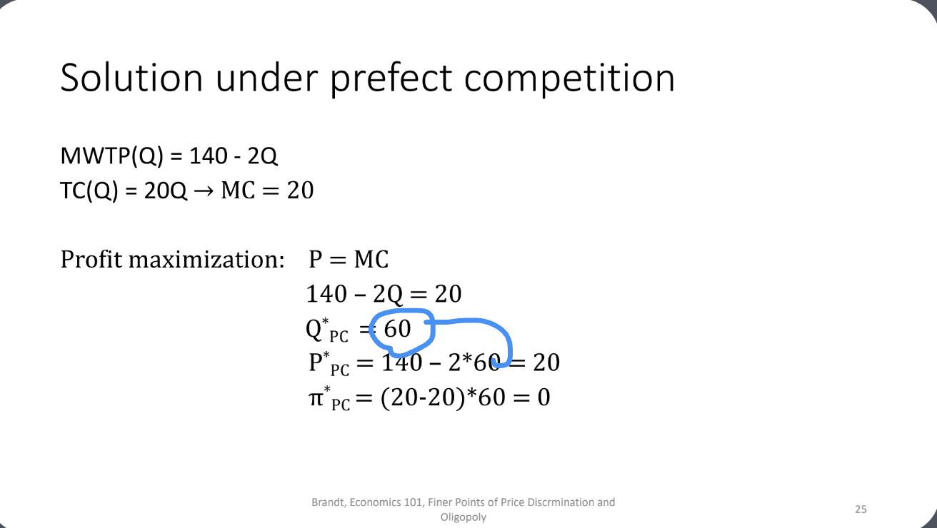
Solution Under Perfect Competition

• MR = MC Standards: Establishment of equilibrium quantity and price under conditions of perfect competition.

• Zero profits indicate an efficient market balancing price and marginal costs.

Page 26

Why Q* PC/2 for Each Firm is Not a NE

• Assessing the incentives for firms to alter their production levels away from proposed equilibrium under competitive pressure highlights the profit-seeking behaviors.

Page 27

Simplified Cournot Framework

• Action Limitations: Two strategic actions for firms, cooperative (to fulfill half monopoly output) versus non-cooperative (higher output).

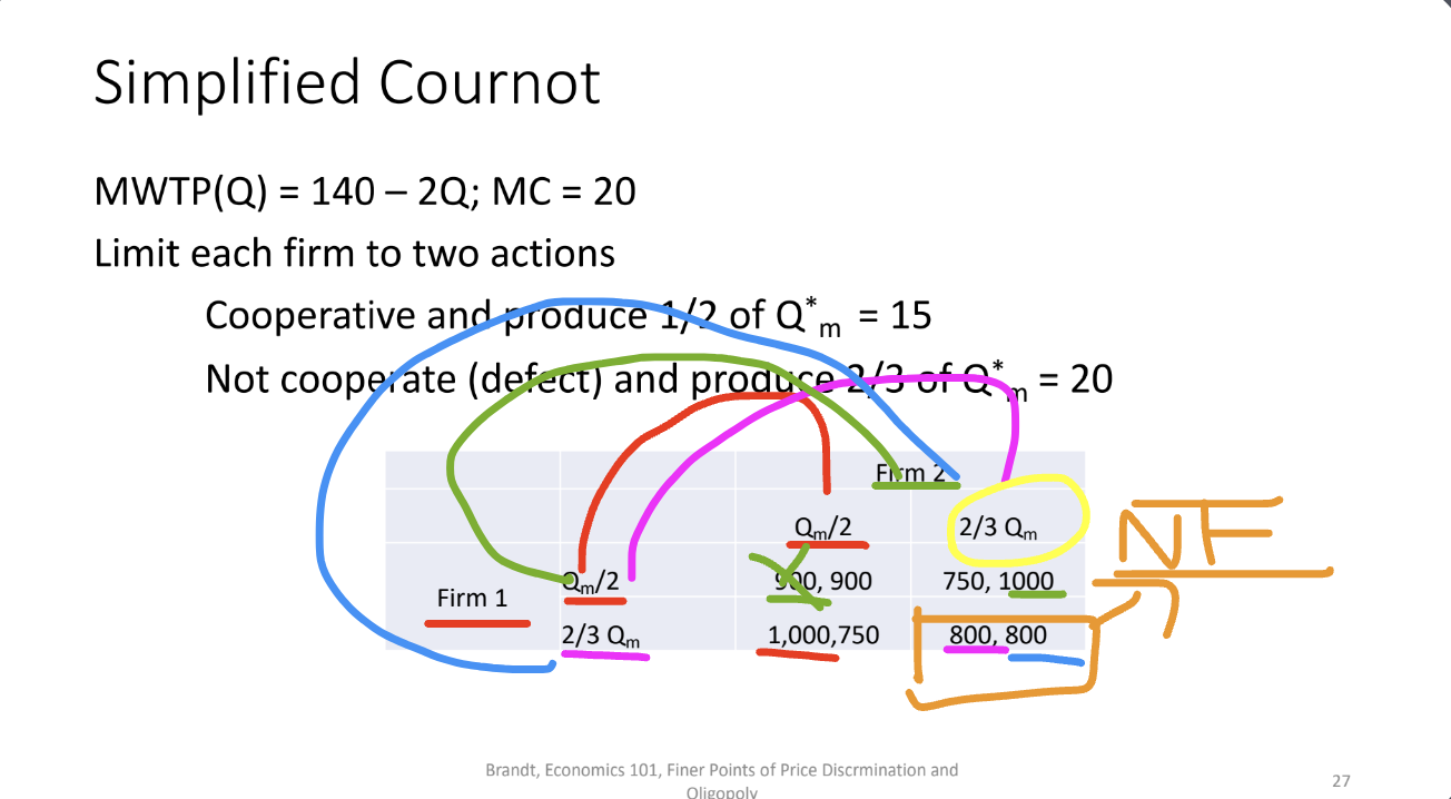
• In a cooperative scenario, firms may agree to restrict their output to increase market prices, while in a non-cooperative scenario, firms compete on quantity, leading to a Nash equilibrium where each firm's output decision is optimal given the output of the other firm.

Page 28

Simplified Cournot Duopoly Outcomes

• Analysis of Strategies: Each player's behavior leads to a dominant strategy similar to the Prisoner’s Dilemma, indicating a unique Nash equilibrium holds.

Page 29

Factors Influencing Collusion

• Difficulties: Legal restrictions, strategic incentives to cheat, and increased complexity with more firms.

• Facilitators: Repeat interactions and structured incentives to support collusion.

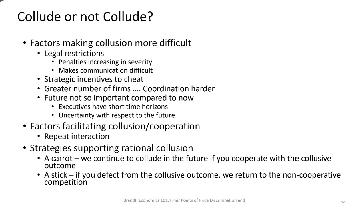
• Market characteristics: Similar cost structures and product offerings can enhance the likelihood of successful collusion.

Page 30

Oligopoly with Varying Assumptions

• Bertrand Assumptions: Firms compete on price under standardized products with consumer tendencies favoring lowest prices.

Firms:

Page 31

Bertrand Paradox

• Marginal Cost Pricing Outcome: Illustrates how just two firms can drive prices down to marginal costs under certain market conditions.

• Resolution Factors: Introduces product differentiation and capacity constraints as critical variables in stabilizing market pricing.