Chapter 7: The Central Limit Theorem
Introductory
- Central limit theorem: If the sample size is large enough then we can assume it has an approximately normal distribution.
- The sample size has to be greater than 30 to assume an approximately normal distribution
- Exponential Distribution: a continuous random variable (RV) that appears when we are interested in the intervals of time between some random events
7.1 The Central Limit Theorem for Sample Means (Averages)
- μX = the mean of X
- σX = the standard deviation of X
- 𝑥¯ ~ N**(𝜇𝑥, 𝜎𝑋 / 𝑛√)** = If you draw random samples of size n, then as n increases, the random variable 𝑥 which consists of sample means, tends to be normally distributed
- sampling distribution of the mean: approaches a normal distribution as n, the sample size, increases.
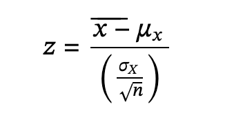
- The random variable 𝑥¯ has a different z-score associated with it from that of the random variable X. The mean 𝑥¯ is the value of 𝑥¯ in one sample.
- μX = the average of both X and x¯
- Standard error of the mean: 𝜎𝑥 = 𝜎𝑋 / √𝑛 =standard deviation of x¯
- Probabilities for means on the calculator
- 2nd DISTR
- 2:normalcdf
- normalcdf (lower value of the area, upper value of the area, mean, standard deviation / √sample size)
- where
- mean is the mean of the original distribution
- standard deviation is the standard deviation of the original distribution
- sample size = n
- Percentiles for means on the calculator
- 2nd DISTR
- 3:InvNorm
- k = invNorm (area to the left of 𝑘, mean, standard deviation / √sample size)
- Where→
- k = the kth percentile
- mean is the mean of the original distribution
- standard deviation is the standard deviation of the original distribution
- sample size = n
7.2 The Central Limit Theorem for Sums
- The central limit theorem for sums: As sample sizes increase, the distribution of means more closely follows the normal distribution.
- ∑X ~ N[(n)(μx),(𝑛√n)(σx)]
- The normal distribution: has a mean equal to the original mean multiplied by the sample size and a standard deviation equal to the original standard deviation multiplied by the square root of the sample size**.**
- The random variable ΣX has the following z-score associated with it:
- Σx is one sum.
- 𝑧 = 𝛴𝑥–(𝑛)(𝜇𝑋) / (√𝑛)(𝜎𝑋)
1. (n)(μX) = the mean of ΣX 2. (√n)(𝜎X) = standard deviation of ΣX
- Probabilities for sums on the calculator
- 2nd DISTR
- 2: normalcdf (lower value of the area, upper value of the area, (n)(mean), (√n)(standard deviation))
- where:
- mean is the mean of the original distribution
- standard deviation is the standard deviation of the original distribution
- sample size = n
- Percentiles for sums on the calculator
- 2nd DIStR
- 3:invNorm
- k = invNorm (area to the left of k, (n)(mean), (√n)(standard deviation)
- where:
- k is the kth percentile
- mean is the mean of the original distribution
- standard deviation is the standard deviation of the original distribution
- sample size = n
7.3 Using the Central Limit Theorem
- Law of large numbers: if you take samples of larger and larger size from any population, then the mean x¯ of the sample tends to get closer and closer to μ.
- Binomial distribution:
- there are a certain number n of independent trials
- the outcomes of any trial are success or failure
- each trial has the same probability of a successful p
Examples