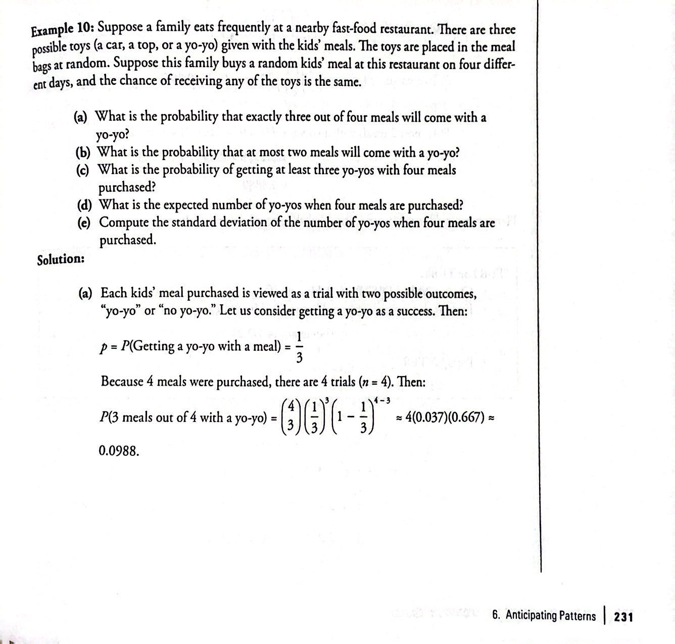
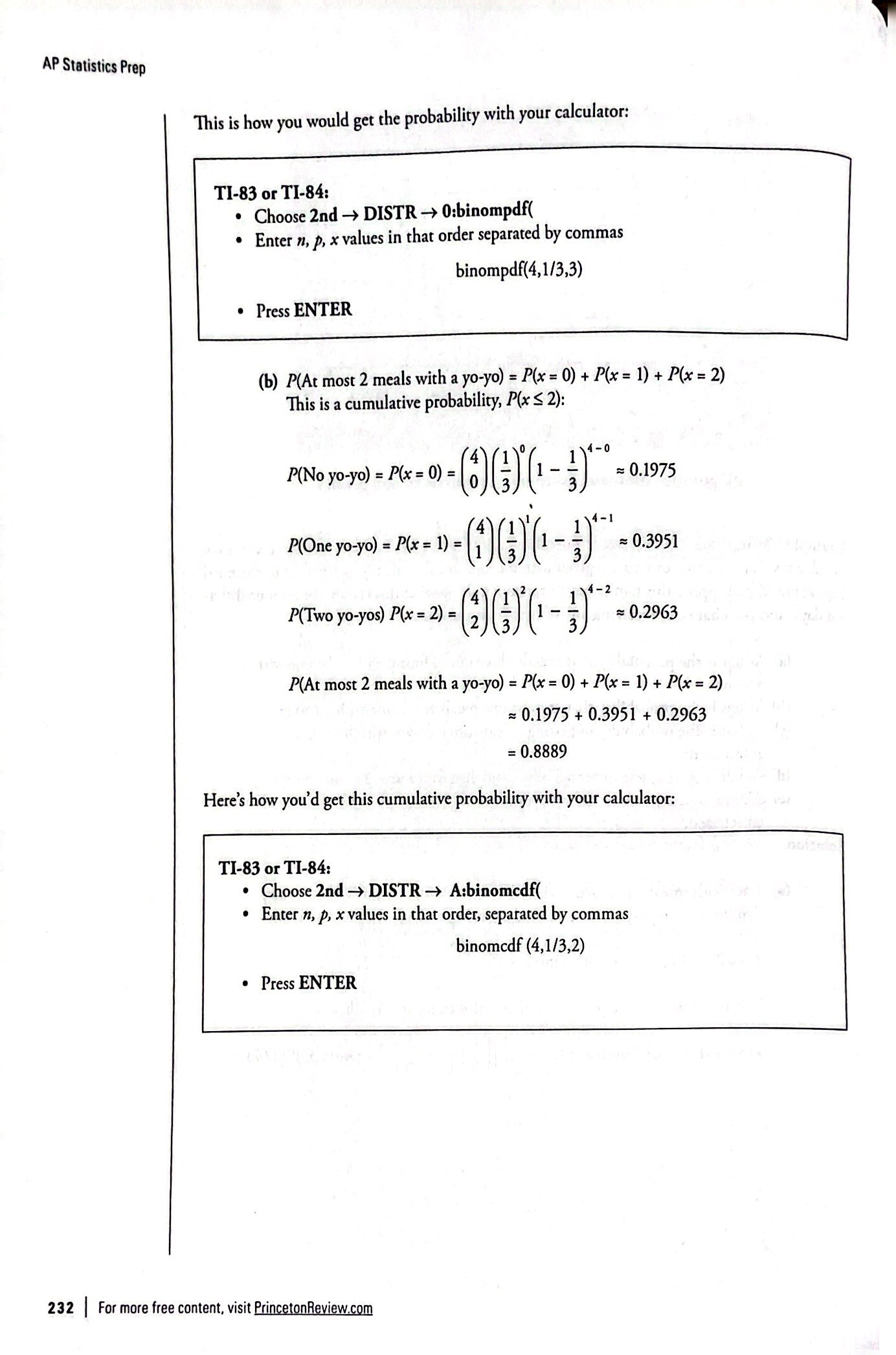
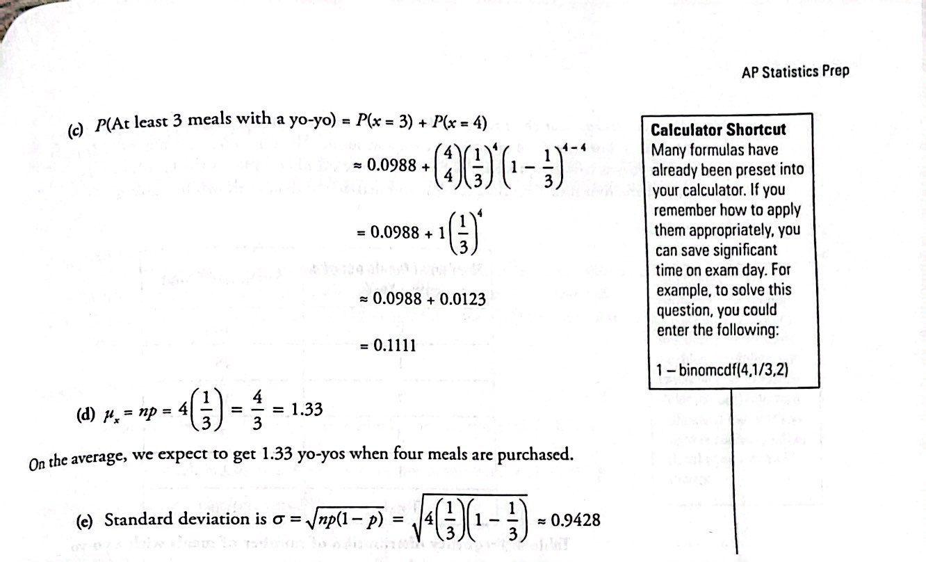
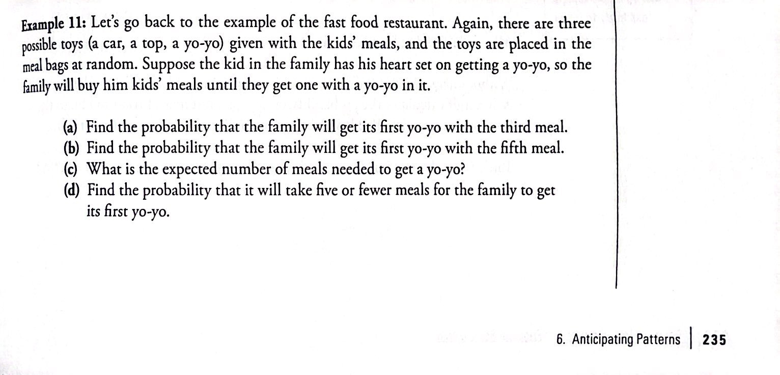
Unit 6: Anticipating Patterns

Terms and Concepts

• Probability: the chance of the outcome of an event
• Sample space: a set of all possible outcomes
• Tree diagram: representation is useful in determining the sample space for an experiment, especially if there are relatively few possible outcomes.

Basic Probability Rules and Terms

• Rule 1: For any event A, the probability of A is always greater than or equal to 0 and less than or equal to 1

• Rule 2: The sum of the probabilities for all possible outcomes in a sample space is always 1

• Impossible event: If an event can never occur, its probability is 0

• Sure event: Of an event must occur every time, its probability is 1

• “Odds in favor of an event”: ratio of the probability of the occurrence of an event to the probability of the nonoccurrence of that event.

  • Odds in favor of an event = P(Event A occurs) / P(Event A does not occur) or P(Event A occurs) : P(Event A does not occur)

• Complement: the set of all possible outcomes in a sample space that do not lead to the event

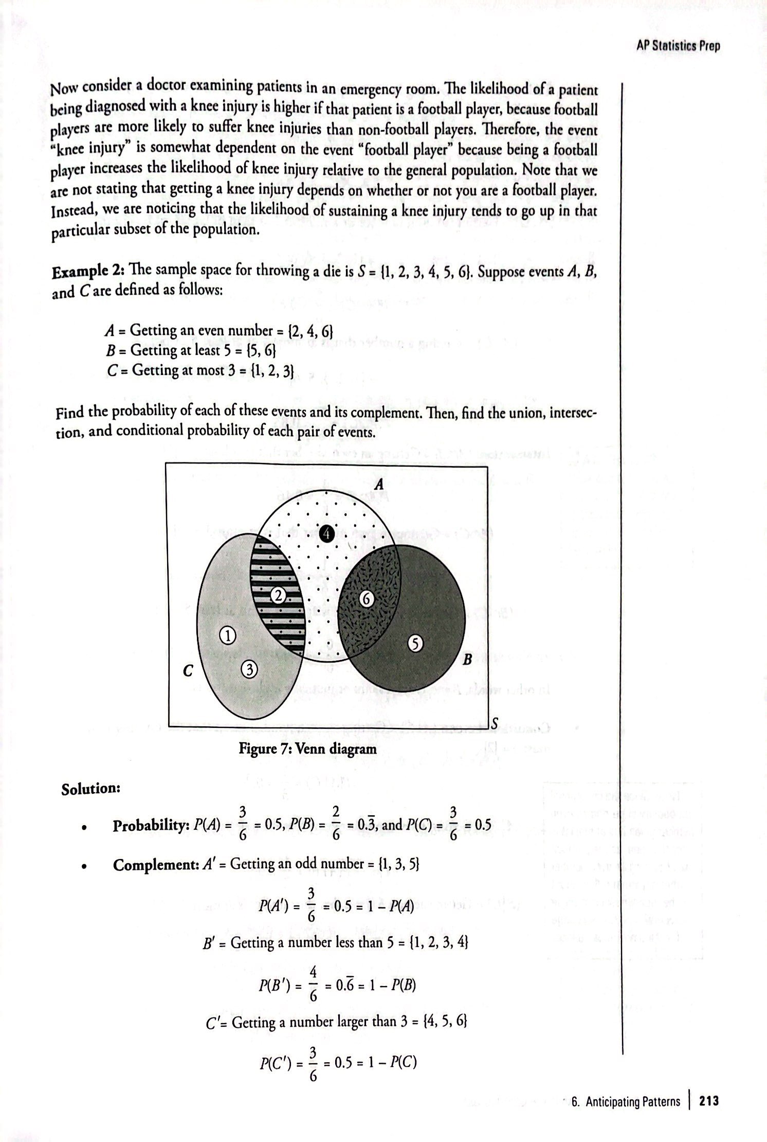
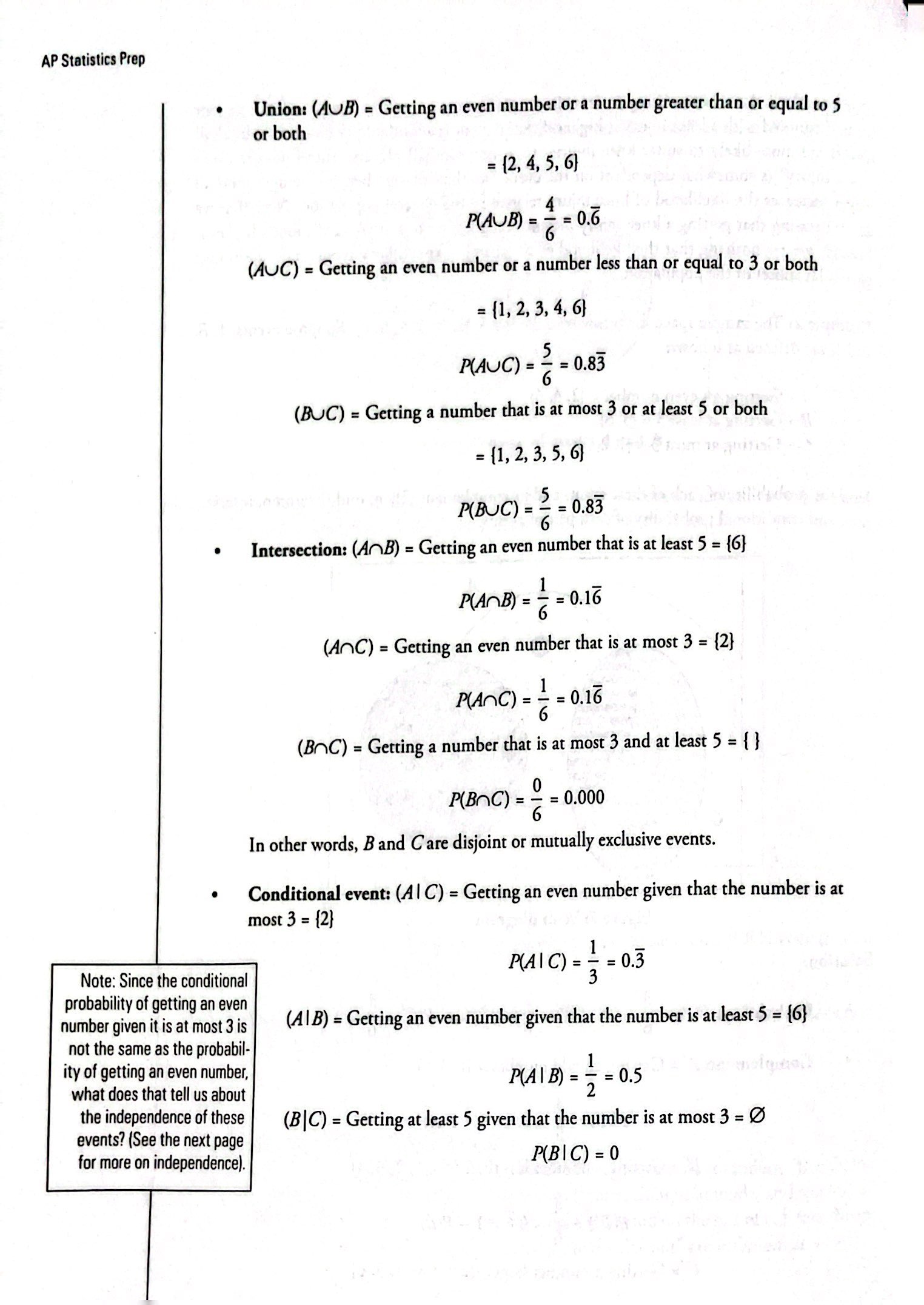
• Disjoint or mutually exclusive events: events that have no outcome in common. In other words, they cannot occur together.

• Union: events A and B is the set of all possible outcomes that lead to at least one of the two events A and B

• Intersection: events A and B is the set of all possible outcomes that lead to both events A and B

• Conditional Events: A given B is a set of outcomes for event A that occurs if B has occurred

  

  

Random Variables and Their Probability Distribution

• Variable: quantity whose value varies from subject to subject
• Probability experiment: an experiment whose possible outcomes may be known but whose exact outcome is a random event and cannot be predicted with certainty in advance
• Random variables: The outcome of a probability experiment takes a numerical value
• Discrete random variable: quantitative variable that takes a countable number of values
• Continuous random variable: a quantitative variable that can take all the possible values in a given range

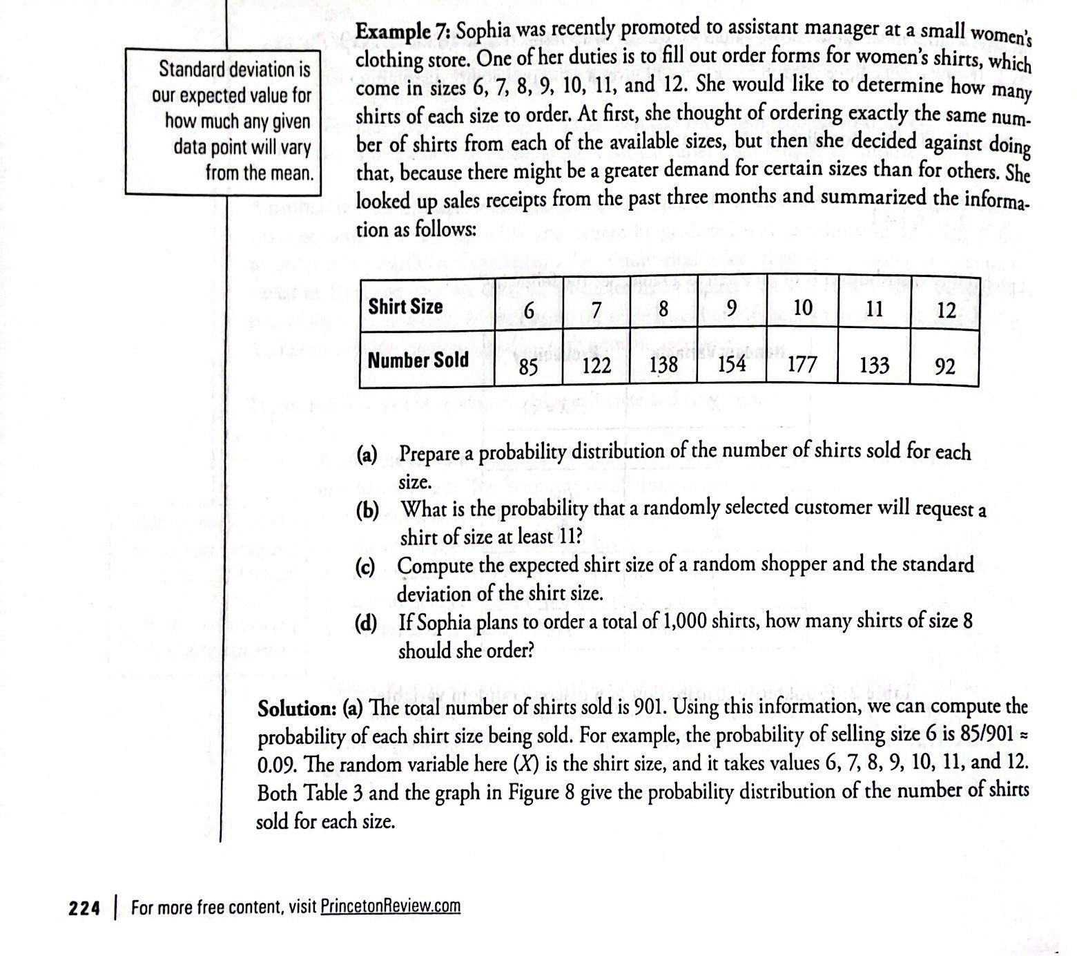
Discrete Random Variable

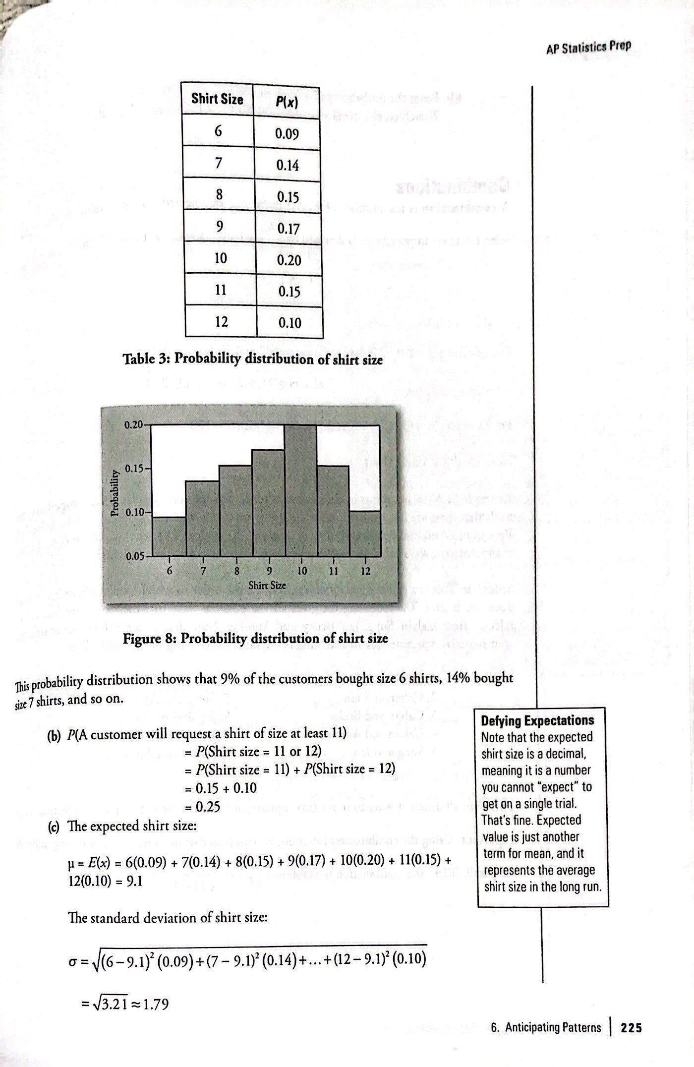
• Expected value: Computed by multiplying each value of the random variable by its probability and then adding over the sample space

• Variance: sum of the product of squared deviation of the values of the variable from the mean and the corresponding probabilities

  

  

  

Combinations

• Combination: the number of ways r items can be selected out of n items if the order of selection is not important.

Binomial Distribution

• 3 Characteristics of a binomial experiment

  • There are a fixed number of trials
  • There are only 2 possible outcomes
  • The n trials are independent and are repeated using identical conditions

• Binomial probability distribution:

  • Mean: μ = np
  • Variance: σ2 = npq
  • Standard deviation: σ = √npq

  

  

  

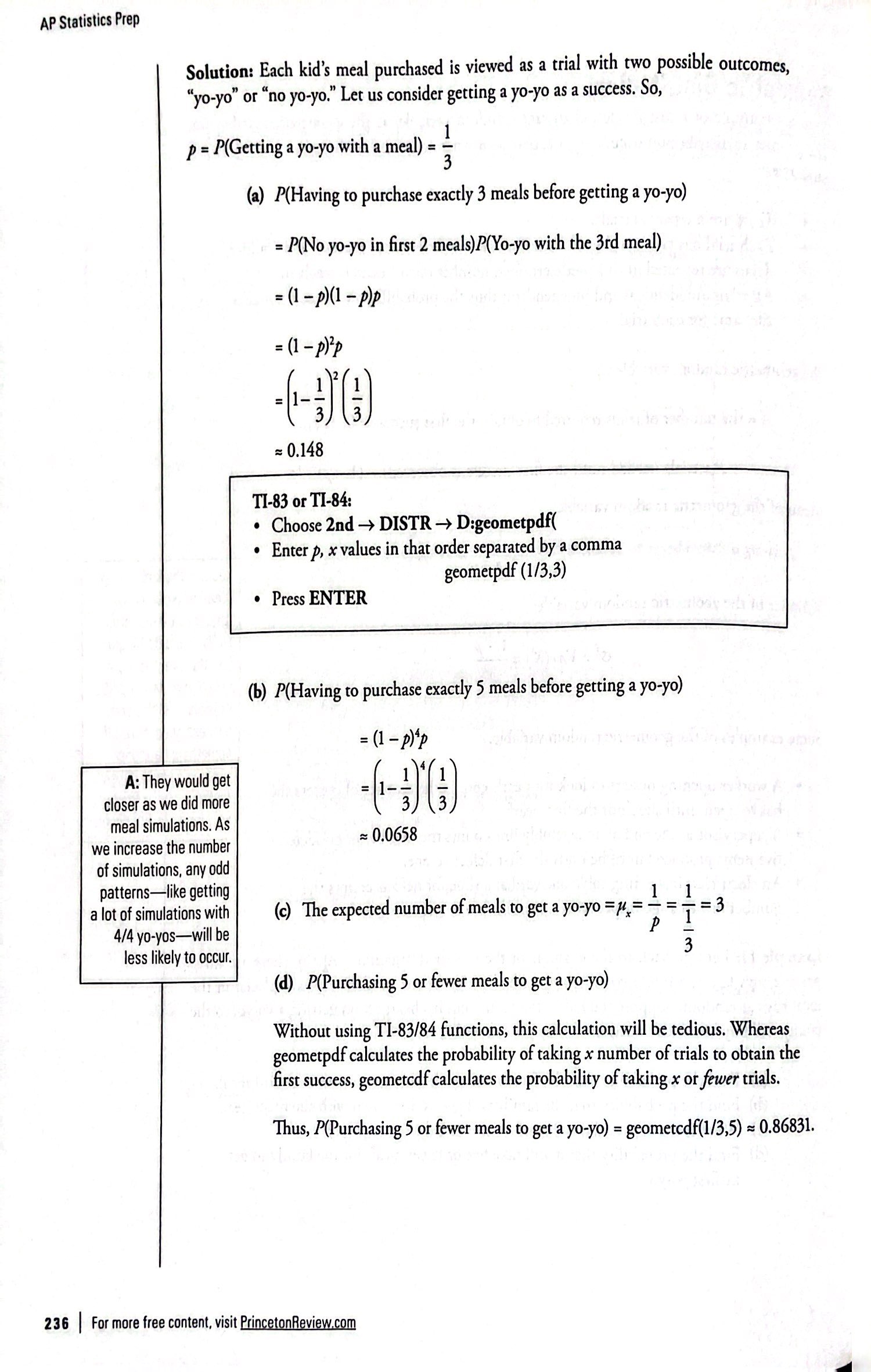
Geometric Distribution

• 3 Characteristics of a geometric experiment

  • There are one or more Bernoulli trials with all failures except the last one, which is a success. In other words, you keep repeating what you are doing until the first success.
  • In theory, the number of trials could go on forever. There must be at least one trial.
  • The probability, p, of a success and the probability, q, of a failure is the same for each trial. p + q = 1 and q = 1 − p.

• X = the number of independent trials until the first success

• Mean: μ = 1/p

• Standard Deviation: σ = √1/𝑝(1/𝑝−1)

  

  

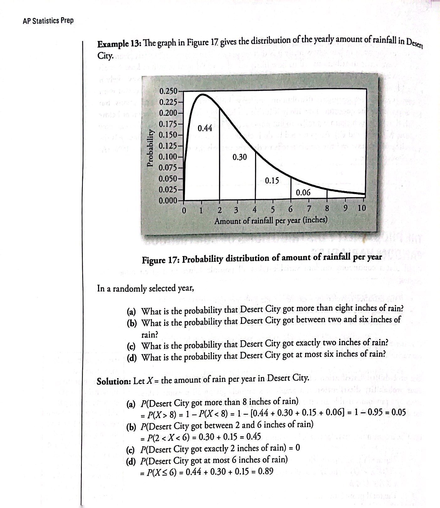
The Probability Distribution of Continuous Random Variables

• The continuous probability distribution (cdf): graph or a formula giving all possible values taken by a random variable and the corresponding probabilities

Let X be a continuous random variable taking values in the range (a, b)

• The area under the density curve is equal to the probability

• P(L < X < U) = the area under the curve between L and U, where a ≤ L ≤ U ≤ b

• The total probability under the curve = 1

• The probability that X takes a specific value is equal to 0, i.e., P(X = x0) = 0

  

Sampling Distribution

• Parameter: a numerical measurement describing some characteristic of a population.

• Statistic: a numerical measurement describing some characteristic of a sample.

• Sampling distribution: the probability distribution of all possible values of a statistic, different samples of the same size from the same population will result in different statistical values

• Standard error: standard deviation of the distribution of the statistics.

  

  

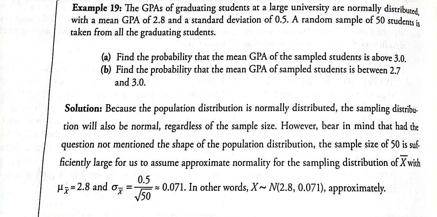
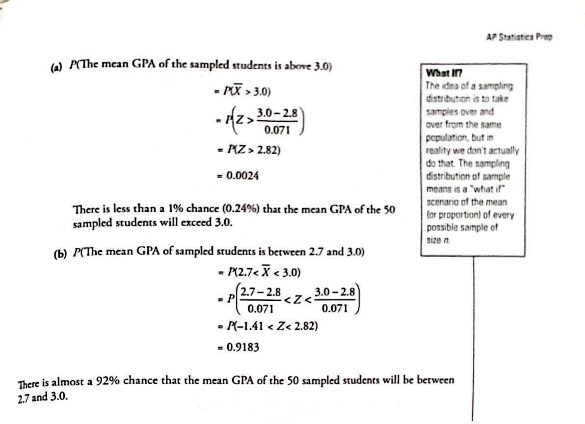
Central Limit Theorem

• Central limit theorem: If the sample size is large enough then we can assume it has an approximately normal distribution.
  • The sample size has to be greater than 30 to assume an approximately normal distribution
• The shape of the distribution of “X bar” becomes more symmetrical and bell-shaped
• The center of the distribution of “X bar” remains at μ
• The spread of the distribution “X bar” decreases, and the distribution becomes more peaked

Calculator Steps

Probabilities for means on the calculator

• 2nd DISTR
• 2:normalcdf
• normalcdf (lower value of the area, upper value of the area, mean, standard deviation / √sample size)
• where
  • mean is the mean of the original distribution
  • standard deviation is the standard deviation of the original distribution
  • sample size = n

Percentiles for means on the calculator

• 2nd DISTR
• 3:InvNorm
• k = invNorm (area to the left of 𝑘, mean, standard deviation / √sample size)
• Where→
  • k = the kth percentile
  • mean is the mean of the original distribution
  • standard deviation is the standard deviation of the original distribution
  • sample size = n

Probabilities for sums on the calculator

• 2nd DISTR
• 2: normalcdf (lower value of the area, upper value of the area, (n)(mean), (√n)(standard deviation))
• where:
  • mean is the mean of the original distribution
  • standard deviation is the standard deviation of the original distribution
  • sample size = n

Percentiles for sums on the calculator

• 2nd DIStR
• 3:invNorm
• k = invNorm (area to the left of k, (n)(mean), (√n)(standard deviation)
• where:
  • k is the kth percentile
  • mean is the mean of the original distribution
  • standard deviation is the standard deviation of the original distribution
  • sample size = n

\
\