Businesses and the Costs of Production (Economics Notes)

Economic Costs, Profits, and the Cost Structure of Production

• Economic costs are the payments that must be made to obtain and retain the services of a resource.

  • Explicit costs: monetary payments.

  • Implicit costs: value of the next best use of a resource (including self-owned resources).

  • Implicit costs include normal profit (the opportunity cost of using entrepreneurial abilities in the production of a good).

  • Non-owners’ resources are included in implicit costs when not paid wages or rents.

• Explicit vs implicit costs and the concept of opportunity costs are essential for understanding economic decisions and profits.

• The standard decomposition:

  • Explicit costs are the accounting costs (only explicit costs).

  • Implicit costs include the opportunity costs (including normal profit).

  • Economic costs = Explicit costs + Implicit costs.

• Economic profit vs accounting profit:

  • Accounting profit = Total Revenue − Explicit Costs.

  • Economic profit = Total Revenue − Economic Costs = Total Revenue − (Explicit Costs + Implicit Costs).

  • Relationship: Economic profit ≤ Accounting profit; a firm can have positive accounting profit but zero or negative economic profit if implicit costs are high.

  • Formulas:
    \text{Accounting profit} = TR - \text{Explicit costs}
    \text{Economic profit} = TR - \text{Economic costs} = TR - (\text{Explicit costs} + \text{Implicit costs})

Short Run and Long Run Production

• Short Run:

  • Some inputs are fixed (e.g., fixed plant).

  • Some inputs are variable (e.g., labor, materials).

• Long Run:

  • All inputs are variable.

  • There is a variable plant, and firms can enter or exit the industry.

• LO1: These distinctions affect cost curves and decisions about scale and entry/exit.

Short-Run Production Relationships

• Total Product (TP): the total quantity of output produced.

• Marginal Product (MP): the change in TP from an additional unit of a variable input (usually labor).

  • Formula: MP = \frac{\Delta TP}{\Delta L}

• Average Product (AP): output per unit of the variable input.

  • Formula: AP = \frac{TP}{L}

The Law of Diminishing Returns

• Assumptions:

  • Resources (inputs) are of equal quality.

  • Technology is fixed.

  • When variable resources (e.g., labor) are added to fixed resources, marginal product eventually falls.

• Rationale: After a certain point, adding more of the variable input yields smaller increases in TP, and MP falls.

• LO2: This law explains the shapes of TP, MP, and AP in the short run.

The Law of Diminishing Returns: Data Snapshot

• A representative illustration with labor input (units of labor) and resulting TP and MP:

  • Labor = 0: TP = 0, MP = —, AP = —

  • Labor = 1: TP = 10, MP = 10, AP = 10.00 (TP/1 = 10)

  • Labor = 2: TP = 25, MP = 15, AP = 12.50

  • Labor = 3: TP = 45, MP = 20, AP = 15.00

  • Labor = 4: TP = 60, MP = 15, AP = 15.00

  • Labor = 5: TP = 70, MP = 10, AP = 14.00

  • Labor = 6: TP = 75, MP = 5, AP = 12.50

  • Labor = 7: TP = 75, MP = 0, AP ≈ 10.71

  • Labor = 8: TP = 70, MP = -5, AP ≈ 8.75

• Interpretation:

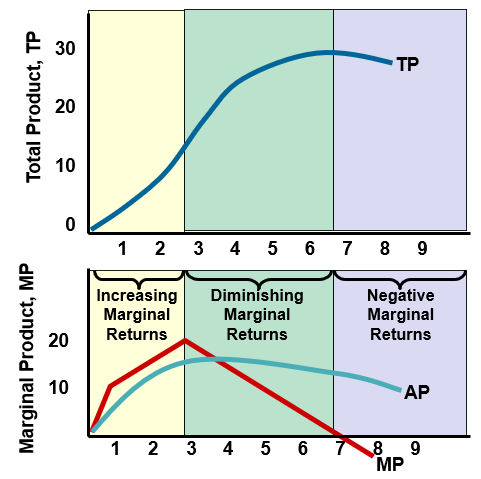
  • MP increases initially (increasing marginal returns), then diminishes, becomes zero, and finally negative.

  • AP initially rises, then falls as more labor is added.

• Visual summary (from the slide set): TP rises, MP initially rises then falls, AP rises then falls; the curve shapes reflect increasing, then diminishing, then negative marginal returns.

• TP, MP, AP relationships (conceptual):

  • Increasing marginal returns when MP rises with more labor.

  • Diminishing marginal returns when MP declines but remains positive.

  • Negative marginal returns when MP becomes negative.

Short-Run Costs: Basic Concepts

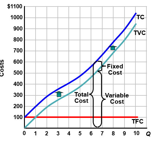
• Short-run costs distinguish between fixed and variable components:

  • Total Fixed Cost (TFC): costs that do not vary with output.

  • Total Variable Cost (TVC): costs that vary with output.

  • Total Cost (TC): sum of TFC and TVC.

  • Formulas:
    TC = TFC + TVC

• LO3: Short-run cost structure underpins most microeconomic analysis of production decisions.
  
  

  

Cost Data and Schedules (Illustrative Tables)

• Per-unit (average) costs:

  • Average Fixed Cost: AFC = \frac{TFC}{Q}

  • Average Variable Cost: AVC = \frac{TVC}{Q}

  • Average Total Cost: ATC = \frac{TC}{Q}

Short-Run Cost Curves: A Quick Picture

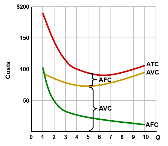
• Average costs by output level:

  • AFC declines as output rises (due to spreading fixed costs over more units).

  • AVC depends on variable costs and may fall initially, then rise due to diminishing returns.

  • ATC is the sum of AFC and AVC and typically falls then rises, creating a U-shaped curve.

  

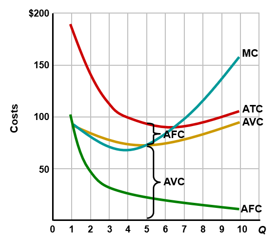
• Marginal cost (MC) generally falls with increasing output in the early range, then rises as diminishing returns set in; MC intersects ATC and AVC at their minimum points in many short-run cost curves.

• Shifts in the curves will occur if either resource prices or technology change.  For example, if fixed costs increase, both AFC and ATC shift up. If labor costs (or some other variable input costs) rise, then the AVC, ATC, and MC would shift up.

  This graph shows the relationship of the marginal-cost curve to the average-total-cost and average-variable-cost curves. The marginal-cost (MC) curve cuts through the average-total-cost (ATC) curve and the average-variable-cost (AVC) curve at their minimum points. When MC is below average total cost, ATC falls; when MC is above average total cost, ATC rises. Similarly, when MC is below average variable cost, AVC falls; when MC is above average variable cost, AVC rises.  Marginal decisions are very important in determining profit levels.  In order to make marginal decisions, marginal revenue and marginal cost are compared. 

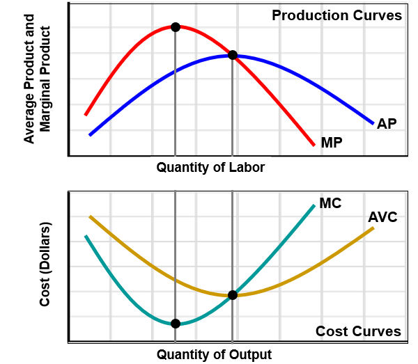
The marginal-cost (MC) curve and the average-variable-cost (AVC) curve are mirror images of the marginal-product (MP) and average-product (AP) curves.  Assuming that labor is the only variable input and that its price (the wage rate) is constant, then when MP is rising, MC is falling, and when MP is falling, MC is rising. Under the same assumptions, when AP is rising, AVC is falling, and when AP is falling, AVC is rising.

Long-Run Production Costs

• In the long run, a firm can vary all input amounts, including plant size.

• All costs are variable in the long run.

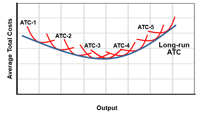
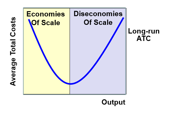
• Long-run average total cost (LRATC) is the envelope of various short-run average cost curves; it shows the lowest possible ATC for any output level when the firm can choose the best scale of production.

Economies and Diseconomies of Scale

• Economies of Scale: long-run cost advantages from increasing the scale of production.

  • Drivers include: labor specialization, managerial specialization, efficient capital, and the advantages of larger-scale production (R&D and advertising can also contribute).

  • Result: LRATC falls as output increases over some range.

  • Economies of scale means, for a time, larger plant sizes will lead to lower unit costs.  An increase in inputs where there are economies of scale will lead to a more than proportionate increase in output. Labor specialization leads to economies of scale because it makes use of special skills; proficiency is gained as the worker concentrates on one task and time is saved.  Managerial Specialization leads to economies of scale because managers can manage more workers with no increased cost, and managers can specialize in their respective area of expertise.  Efficient Capital leads to economies of scale because high volume production warrants the expensive large scale equipment.  Other factors lead to economies of scale because costs such as Research & development, and advertising are spread out over larger quantities.

    Constant returns to scale will occur when ATC is constant over a range of output.  When there are constant returns to scale, an increase in inputs will result in a proportionate increase in output.

• Diseconomies of Scale: long-run cost disadvantages from increasing the scale of production.

  • Causes include: control and coordination problems, communication problems, worker alienation, and shirking.

  • Result: LRATC rises as output increases beyond a certain point.

• Constant Returns to Scale: LRATC remains constant as output expands.

• MES (Minimum Efficient Scale):

  • Definition: the minimum level of output at which long-run average costs are minimized.

  • Role: can determine the structure of the industry (whether many small firms or a few large firms dominate).

  MES helps explain industry structure and scale decisions across industries.

• Long-run vs short-run cost curves (conceptual):

  • The long-run ATC curve is formed by the lower envelope of the various short-run ATC curves at each output level.

  • In practice, SRATCs correspond to different plant sizes; the LRATC picks the most cost-efficient plant size for a given output.
    

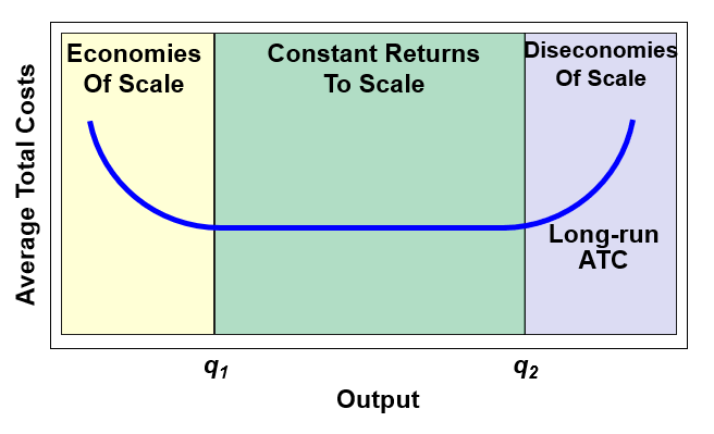
This is a long-run ATC curve showing industries with an extended range of constant returns to scale.  These industries will be populated by firms of many different sizes. Small and large scale producers will coexist and be equally successful.  MES occurs at an output of q₁.

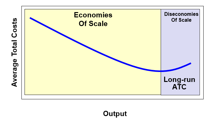
Industries with economies of scale over a wide range of outputs will lead to a few large scale firms.  The long-run ATC curve is lowest only when there is a large output. 

This is a long-run ATC curve where economies of scale exist, are exhausted quickly, and turn back up substantially.  Here minimum efficient scale occurs at a very low level of output.  This results in a large number of small producers.

Applications and Illustrations

• Rising gasoline prices can raise short-run costs for firms with fuel-intensive operations (e.g., FedEx). AVC, MC, and ATC all to rise for firms that use this type of energy as an input. As a result, firms like FedEx will see substantial cost increases whereas firms that do not need to transport products physically will not be affected by the rise in fuel costs.

• Successful start-up firms (e.g., Starbucks) illustrate scale and efficiency considerations in real-world settings. Start-up firms have been successful by lowering their ATC as they increased output and achieved economies of scale.  This spreads out R&D and advertising costs over a larger number of units.  Some examples of these types of firms are Starbucks and Google.

• Manufacturing examples (e.g., Verson stamping machines & aircraft production) show how capital intensity and learning-by-doing impact costs.

• Ready-mixed concrete plants illustrate economies of scale in construction-related industries.

Sunk Costs and Decision Rules

• Sunk costs: costs that have already been incurred and cannot be recovered.

• Rule: Do not engage in any activity where marginal benefit (MB) < marginal cost (MC).

• Rule: Ignore sunk costs since they are irrecoverable.

• These principles guide rational decision-making beyond the sunk-costs consideration.

  Sunk costs are irrelevant in decision-making. An example of a firm’s sunk cost might be when a firm spends a lot of money researching and developing a new product, but once the product reaches the market, it is a flop.  Should the firm continue to produce the product? In making a new decision, you should ignore all costs that are not affected by the decision.  R&D, marketing, and production costs for a product that has insufficient demand should be considered sunk costs. The firm should discontinue production of the product. E.g. Pfizer’s decision to withdraw its novel insulin inhaler (pretax loss of $2.8b)

• Quick recap of key formulas:

  • Economic profit: \text{Economic profit} = TR - (Explicit\ costs + Implicit\ costs)

  • Accounting profit: \text{Accounting profit} = TR - Explicit\ costs

  • MP: MP = \frac{\Delta TP}{\Delta L}

  • AP: AP = \frac{TP}{L}

  • TFC, TVC, TC: TC = TFC + TVC

  • AFC, AVC, ATC: AFC = \frac{TFC}{Q},\quad AVC = \frac{TVC}{Q},\quad ATC = \frac{TC}{Q}

  • MC: MC = \frac{\Delta TC}{\Delta Q}

• LO1–LO4: The notes cover learning objectives related to cost concepts (economic vs accounting costs, explicit vs implicit costs), short-run vs long-run distinctions, production relationships (TP, MP, AP) and the law of diminishing returns, cost curves (TFC, TVC, TC; AFC, AVC, ATC, MC), LR costs, economies/diseconomies of scale, MES, and practical implications including sunk costs.