W2: Introduction to MRI
Topic 1: Basics of image formation in MRI
Goal: Familiarization with MRI terminology
Hardware components used MRI for human brain scanning
⚠ MRI can be used to investigate various organs although it mainly focuses on human brain imaging.
Receiver (or head) coil detects/receives signals from the brain
Transmitter coil produces said signal
Gradient coils, which surround transmitter coil, are essential to localize signals.
Gradient coils are small electromagnets that can alter the magnetic field strength.
Main magnetic field, measured in Tesla units, surrounds the receiver coil, transmitter coil and gradient coils
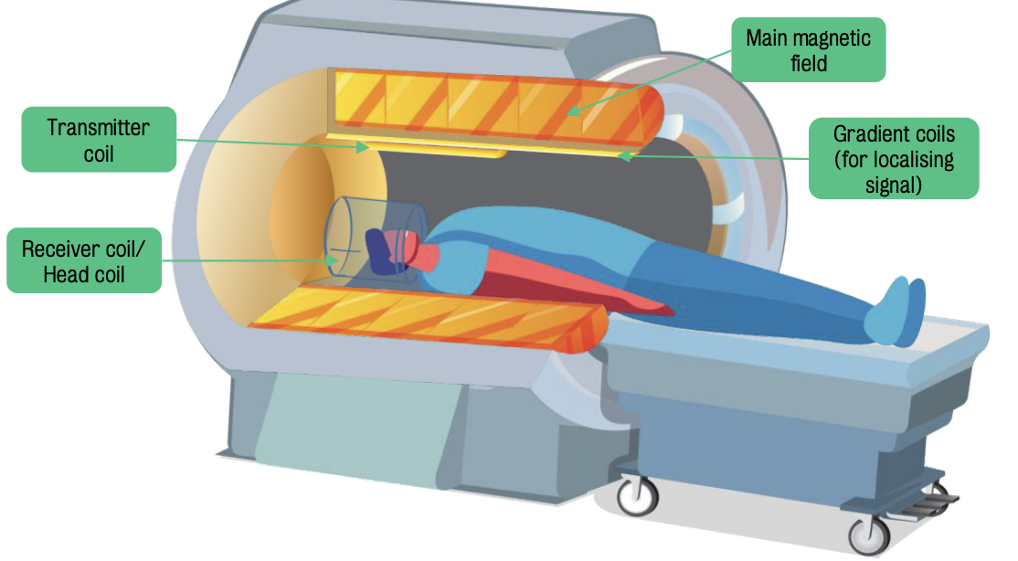
Clinical scanners have field strengths of 1.5 T, while research scanners have field strengths of 3T or above.
⚠ This is at least 104 x higher than Earth's magnetic field (0.5 micro Tesla).
Higher magnetic field strengths improve performance but are more expensive to manufacture.
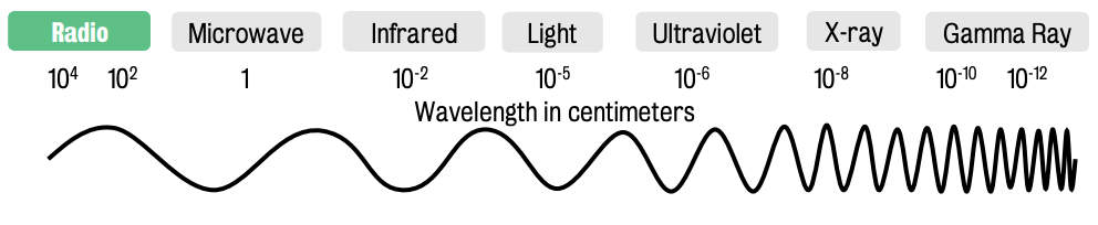
Basic principles of magnetic resonance imaging deals with interaction between certain atomic nuclei.
Radiofrequency (at the left) energy is part of the electromagnetic spectrum.
Waves (on that spectrum) are defined by wavelength and frequency
Wavelength = distance between peaks of the wave
Frequency = cycles per second
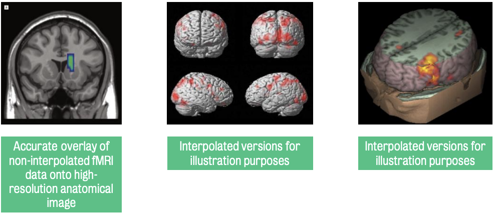
Pixel (picture + element) = single point on a computer screen
Voxel = 3D pixel
MR images are made up of a series of voxels that correspond to a volume of tissues
MRI scanners are designed to measure the signal generated by each voxel & localize them to create recognizable images.
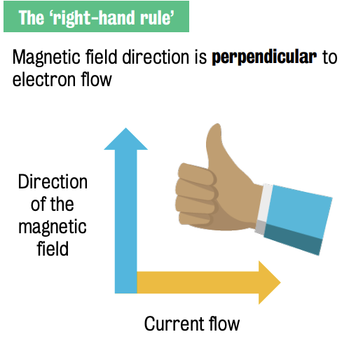
Basic principles of electromagnetism
Direction of the magnetic field defined by the ‘right-hand rule’
For MRI purposes, only the hydrogen protons in the nucleus are of interest.
Hydrogen proton rotates on its axis & is positively charged
Protons act as tiny bar magnets, abundant in the human body due to water content.
MRI can measure the signal from these protons.
⚠ Fats, carbohydrates and proteins also contain protons and so together they can sum to produce a detectable signal.
In the absence of a strong magnetic field protons are randomly aligned and essentially cancel each other out.
This random alignment cancels out magnetic effects in normal conditions
In the presence of a strong magnetic field protons align with or against the magnetic field.
No in-between states.
Protons precess like gyroscopes in a magnetic field, tracing circular paths.
Rate of precession is proportional to the strength of the magnetic field.
This relationship is defined by the Lamor equation
:. protons ‘precess’ about their axis at the frequency described by the Larmor equation.
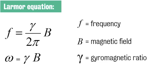
Radiofrequency (RF) pulses — which are electromagnetic pulses — are applied at the Larmor frequency (i.e., frequency of precession) to create MR images.
Larmor frequency for a 1.5 T scanner is just under 64 MHz; for a 3 T scanner, it's about 128 MHz.
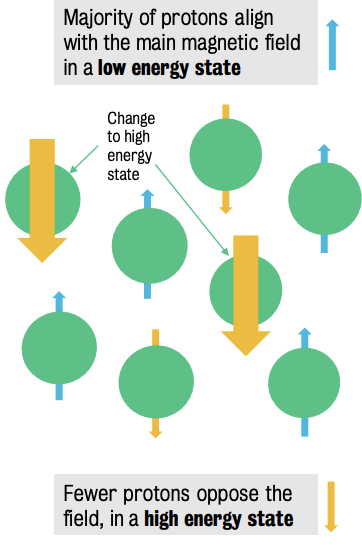
Longitudinal magnetization
Involves cancelling opposing vectors
Can not be detected but only be inferred.
In a 1T magnetic field, protons have a Larmor frequency (precession frequency) of 42.58 MHz.
Transmitting a radio frequency pulse at this frequency causes protons to absorb energy and move to the high-energy state.
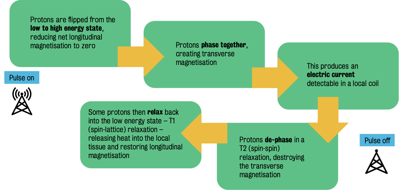
By providing the right amount of energy to flip 50% of the protons, the net longitudinal magnetization reduces to 0, nullifying magnetic forces.
Resonance component of MRI
Transverve magnetization = net magnetic force created horizontally or perpendicular to longitudinal magnetization (when all magnetic fields are combined.
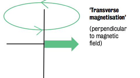
Just as a current can create a magnet, a magnet can create a current.
Sinusoidal radiofrequency pushes protons to spin in synchrony, creating a creates a sinusoidal wave
Rotating magnetic field in MRI generates measurable alternating current in a coil of wire
Protons will de-phase as positive charges repel each other, :. reducing net transverse magnetization to 0 (T2 or spin-spin relaxation)
No net energy transfer occurs during this de-phasing process.
T1 or spin-lattice relaxation = relaxation process involving high-energy protons transitioning to a lower energy state, releasing absorbed energy as heat to the surrounding tissue.
Different tissues in the brain (grey matter, white matter, CSF) have differences in their T1 and T2 relaxation times.
Topic 2: Basics of image localization in MRI
⭐ ️During T1 relaxation process, the energy released is converted to heat transmitted to local tissues and longitudinal magnetisation is restored.
RF pulse at Lamor frequency flips protons from a low to a high energy state, causing them to synchronize and move the longitudinal magnetization into the transverse plane.
Contrasting tissue types
Brain tissue-specific differences in T1 and T2 relaxation allow us measure differences by changing how quickly we stimulate tissue [TR or repetition] & listen for the signal emitted by precessing protons [TE or echo time]
TR and TE are adjustable parameters that can manipulated to maximize signal of interest (i.e, create contrasts in MRI images)
:. T1 and T2 relaxation times are properties of tissues we wish to image
Form pulse sequence
Dephasing (i.e., moving out of synchrony) of fat protons occurs ++ quickly due to the more rigid structure.
Quicker dephasing of protons is a consequence of rapid T2 relaxation
T1 relaxation also occurs more quickly in fat & energy is released in the form of heat, allowing longitudinal magnetization to re-grow.
Water (H20) maintains transverse magnetization longer than fat due to its less rigid structure.
High-intensity signals from water appear bright on a grey scale, while low-intensity signals from fat appear darker.
Transverse magnetization generates an electric current in a local coil, but as protons de-phase through T2 (spin-spin) relaxation, the transverse magnetization diminishes.
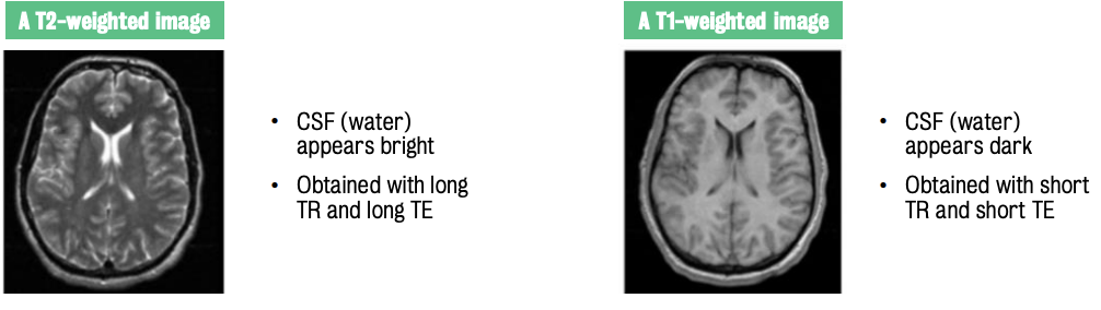
T2-weighted images highlight CSF as bright, while T1-weighted images show CSF as darker.
Localization in 3D space
Ultimate goal of MRI = localization of signal into 3D space, i.e. knowing which part of the brain is generating signal we are measuring.
Main (or static) magnetic field (B0)
Reported in units of Tesla (T)
Strength ranges between 1.5 and 7T & determines Larmor frequency
Static field is uniform in strength across the whole board of the scanner; = homogenous
Three gradients magnets (known as the gradient coils) allow us to localize signal within the scanner in 3D space.
Slice gradient (Gs)
varies the strength of the magnetic field along the y axis
Field strength increases as you move towards the feet and decreases as you move towards the head
Changing field causes protons to precess at different frequencies depending on their y-axis position
Phase-encoding gradient (Gp)
Field strength increases from left to right
Protons to precess at different frequencies depending on their x-axis position
Frequency-encoding gradient (Gr)
Varies field strength from bottom to top (i.e., along the z-axis)
⭐️ Together these gradient coils allow us to finely tune the strength of the magnetic field across all 3 dimensions.
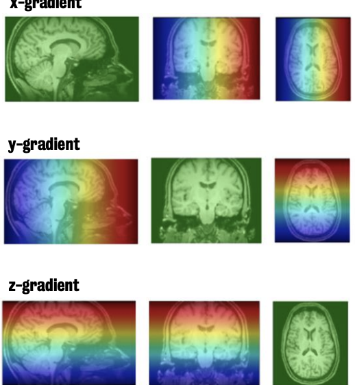
Note: Hotter colours = higher field strengths; colder colours = lower field strengths
How to localize a signal
Localize a slice in the brain
By transmitting a radio frequency pulse at just the right frequency (F3) we can “excite” a single slice of brain
Localize a line
By exciting a specific slice, slice gradient is switched off and phase encoding gradient is switched on, creates another magnetic gradient across the excited slice of the brain → each ‘line’ of protons within the slice returning energy at a different phase
Localize a unique voxel
Frequency encoding gradient is switched on.
Final induces a third magnetic field
Gradient impacts on the precession frequency of the protons within each slice
Frequency encoding phase allows for signal to be localized in 3D space.
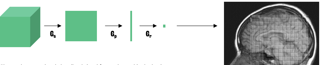
:. By using gradient coils to massage the main magnetic field in 3 dimensions, we can localize our signal to a discrete region within the brain.
Topic 3: Neuroimaging analysis
Goal: ① Discover various types of neuroimaging data; ② how we analyze neuroimaging data ③ common analytical challenges
What are neuroimaging data made of?
Pixels are the basic building blocks of 2D images.
Dimensions: width (x-axis) & height (y-axis)
Images are made up of darker & lighter pixels. This shade is called grey level (intensity value)
The darker the pixel, the higher the intensity value.
Image properties:
Matrix size refers to the size of the pixel grid
Image width x image height (usu. 64 × 64 voxels)
Pixel refers to the dimension of the pixel itself
Pixel width x pixel height (usu. 3.75 mm2)
Field of view (FOV) represents the size of the grid
Measured in cm
Can be calculated using matrix size and matrix size values (image dimensions x pixel dimensions)
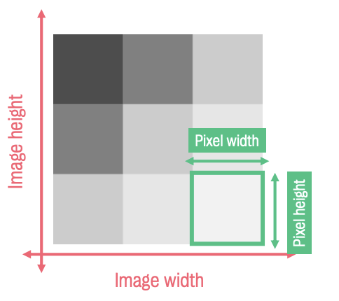
3rd dimension (z-axis) is referred to as slice thickness
Voxels (volume elements) are the 3D equivalents of pixel
fMRI
Based on contrasting brain activity between experimental tasks
In acquiring fMRI data, brain volumes are captured every few seconds during an experiment.
⚠ We do not scan the whole brain at once for fMRI, we acquire slices and reconstruct the brain afterwards by stacking these slices
Understanding the methods section in neuroimaging papers is crucial to draw out information about MRI acquisition parameters and image properties
Challenges associated with neuroimaging data analysis include noise and the need to correlate brain activity with experimental tasks.
fMRI data is usually stored in a 4D file
Two main conventions used to store data within a 4D file:
XYZ-T orientation: 3D brain volumes are simply stored one after another
XYT-Z orientation: Image format the data are stored slice by slice
Time series = basic building blocks of all the analyses
Generated by extracting and plotting the intensity values for a specific set of coordinates
Types of imaging
In qualitative imaging (e.g. fMRI), voxel intensity values are arbitrary and do not represent real physical quantities, while in quantitative imaging (e.g., T1 & T2 mapping), these values correspond to actual tissue properties.
In qualitative imaging, voxel intensities vary between scanners (equipment)/sessions/centres while they remain consistent in quantitative imaging.
Spatial resolution refers to the detail in images, where higher spatial resolution corresponds to smaller voxel sizes, allowing for more detailed imaging.
Higher spatial resolution, the more details.
MRI-based techniques have the highest spatial resolution (esp. structural and anatomical imaging).
Temporal resolution refers to the speed of data acquisition, with fMRI data typically having a temporal resolution in the seconds (s) range.
We only acquire a snapshot of brain activity every couple of seconds.
EEG and MEG have the highest temporal resolution, enabling fast brain processes invisible under other techniques (e.g., fMRI)
⚠ It is important to select appropriate imaging techniques based on specific research questions and the inherent trade-offs between different imaging modalities.
Neuroimaging Data Analysis
1st level refers to subject level analysis
2nd level: group level analysis
3rd level: blob map
Pre-processing refers to cleaning up the data
It is primordial to go through pre-processing stage before conducting statistical analysis
Main aim: increase signal to noise ratio (SNR) — i.e., having as much of signal as possible and as little noise as possible.
Involves removing sources of noise — i.e., the detrimental effects of head motion, background noise, physiological noise (e.g., heart beat, breathing)
Brain anatomy variability is taken care off by smoothing (i.e., blurring) the data and normalize into a standard reference template
Other modality-specific artefacts (e.g., the use of diffusion tense imaging (DTI) for cleaning up eddy currents)
Anatomy will differ :. to diminish the impact of brain viability, pre-processing is crucial.
Derek Jones’ data processing experiment — where he invited colleagues to analyze data using an online DTI dataset — highlights that neuroimaging data analysis is not an exact science
Results indicated a big source of variance from pre-processing stage of the analysis
:. it is important to acknowledge different pre-processing options, different orders and settings to choose the best practice before statistical analysis
⚠ Always employ the plural when referring to data. We say “the data are…” and not “the data is…”
Analysis scope
Important to choose between Whole brain analysis or Region(s) of interest (ROIs) analysis based on the presence of a clear hypothesis
ROIs are the standard choice in the presence of an hypothesis as it focuses on a small number of regions, meaning less voxels to deal with.
Whole brain analysis may → multiple comparisons problem
Pre-registering study online helps avoiding deviations from original hypothesis
ROIs choice (i.e., choosing region of interest) can be made using methods, including:
Structural definition
Based on an anatomical atlas (e.g. e homunculus or all the sensory-motor regions)
Theoretical basis (e.g., paper or book)
Meta-analysis
Functional definition (localiser scans)
i.e., quick fMRI experiment to define precisely in each of your participants where your region of interests are
Avoid over-selling the results of exploratory analysis & circularity (double-dipping) if employing both whole brain analysis and ROIs
The number of values per voxel depends on the modality
Student’s t-test = statistical test used to compare values per voxel (1 value/voxel)
The imager’s fallacy is a statistical problem that persists in modern day
Saying that two results are the same or different by just looking at them side by side 🚫
Discrepancy to the naked eye hold no statistical validity
✅ Statistical comparison between the images is needed reach to reach a conclusion (of statistical difference — or not).
Parametric vs non-parametric test
Renewed interest in the use of non-parametric statistics in neuroimaging following the publication high-impact papers and blog posts
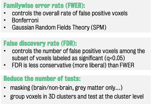
Multiple comparisons problem:
When doing multiple t-test, a single p-value is insufficient
Bonferroni correction (usu. solution for this problem) cannot be used in the context of neuroimaging.
It is a correction for independent tests and :. far conservative and far too harsh
Instead, further data exploration is recommended
Potential pitfalls in neuroimaging:
Type 1 errors — statistical anomalies which arise when one does not correct for multiple comparison
Running tens of thousands of statistical tests
Dead salmon experiment (2012 Ig Nobel Prize Winner in Neuroscience)
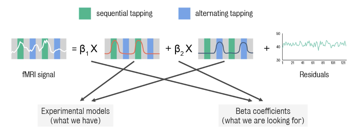
Final part of neuroimaging analysis: Data modelling
Presence of an (usable) experimental model →general linear model
Other model free approaches — in the absence of an experimental model or an aversion towards present one:
Independent component analysis (ICA)
Principal component analysis (PCA)
Machine learning (SVM or Gaussian processes)
ICA is a pattern-matching technique that decomposes the signal onto subcomponents regrouping all the voxels that behave in the same way :. all brain regions are synchronized.
In resting state fMRI, this enables ICA to discriminate the various brain networks that are activated when the brain is at rest.
Famous e.g.,: default mode network (signature of brain at rest)
Echoes = other networks who map onto relevant task-related networks
Machine learning (artificial intelligence) finds patterns in a set of training data and uses these to classify the data either in binary classes.
Produces maps of discriminative regions (similar to blob maps)
Enables predictions based on training
In neuroimaging, machine learning is being used in an increasing number of fields from depression to autism via psychosis to predict treatment response and psychosis development.