Lecture 1 - Video notes

Welcome to Psych 234

Importance of Regression

• Regression Methods: Essential for final year project flexibility in testing hypotheses and analyzing data.

• Types of Predictors:

  • Continuous and categorical predictors can be modeled simultaneously.

  • Example: ANOVA requires transforming continuous variables into categorical variables for analysis.

• Secondary Variables: Regression handles extraneous or nuisance variables, allowing their effects to be partialled out when investigating primary predictors.

• Interaction Effects: Understanding how different predictors influence each other can enhance the model's accuracy and provide deeper insights into the data.

Advantages of Regression

• Flexible Hypothesis Testing: Uses null hypothesis significance testing with p-values.

• Power: Retains higher statistical power than ANOVA due to individual-level analysis.

• Predictive Capability: Generates predictions from observed data using regression equations, aiding future research hypothesis development.

• Extensions: Capable of handling various data forms, including binary, ranked, and longitudinal data.

• Flexibility - regression allows for various statistical modeling options , enabling researchers to tailor their analyses to specific research questions and data characteristics.

• Statistical power - increase te ability to detect effects if they exist

• Prediction - regression models facilitate making prediction based on data set variables

  • interactions: Understanding how variables work together is crucial for accurate predictions.

  • Mathematics Preparation: Expect some mathematical engagement in analysis.

• Extensions - more complex regression model can extend basic findings

Data Preparation and Model Interpretation

• Data Preparation: More necessary when mixing variable types (categorical and continuous).

• Intercept Term: Important for accurate model interpretation; varies based on predictors.

  • Intercept Term: Key to modeling; signifies average outcome when all predictors = 0.

  • Considerations: Understanding its role is crucial for interpretation.

• Reference Levels: Knowledge from ANOVA regarding categorical predictors will aid in regression analysis.

  • Reference Levels: Essential for categorical variables and their impact on outcome.

  • Complexity: Emphasizes understanding how variables interact.

Upcoming Focus Areas

1. Week 11: Review of correlation, simple and multiple regression.

2. Weeks 12-13: Categorical and continuous variable modeling, understanding and manipulating intercept terms, exploring interaction effects.

3. Week 14: Mediation models for inferring causality.

4. Week 15 (Half): Variable reduction with factor analysis (not in class test).

5. Weeks 17-19: Logistic and ordinal regression.

6. Week 20: Class test (58 MCQs, 12 R analysis questions).

Learning Resources

• Multiple-choice quizzes: Non-graded; три attempts per quiz.

• Recommended Reading: Howell's "Fundamental Statistics for the Behavioral Sciences" (Chapters 9-11).

Review: Correlation and Regression Concepts

Correlation (Pearson's r)

• Properties: Strength and direction of relationship between two continuous variables (Range: -1 to 1).

• Types of Relationships:

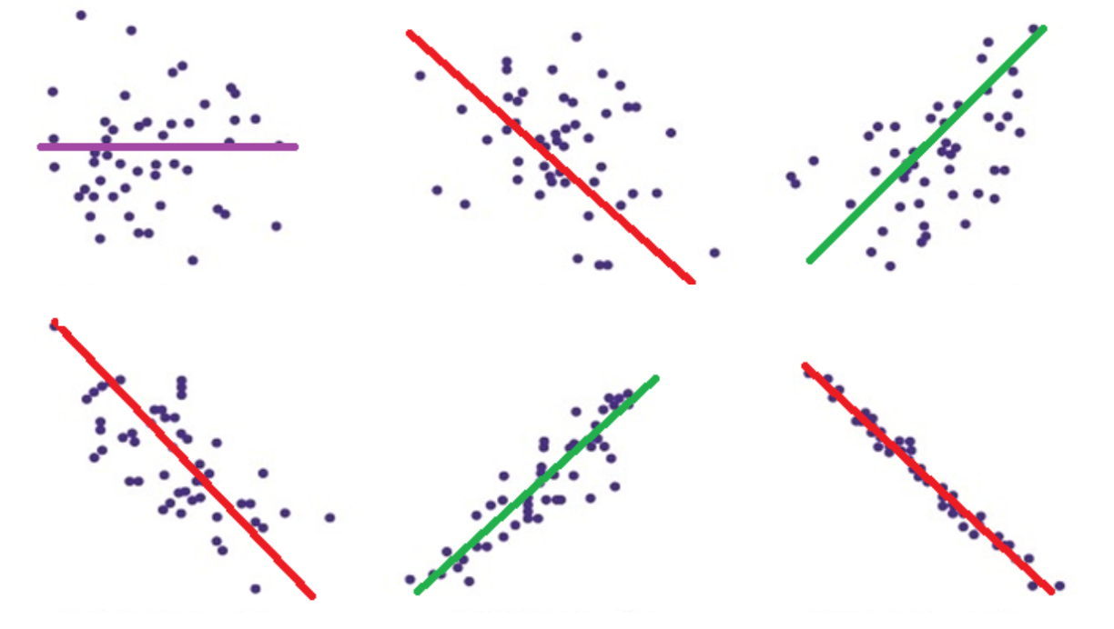
  • Negative Relationship: x ↑ while y ↓ (or vice versa).

  • Positive Relationship: x ↑ and y ↑.

  • No relationship : x remains constant while y fluctuates.

• Strength represented by proximity to +/- 1 in scatterplots.

• The magnitude of a number tells us the strength of a relationship

• Values that are closer to -1 or 1 detonate a stronger relationships while values that are closer to 0 detonate an absence of a relationship

• Strength is denoted by how close the data points are to the line of best fit

• In summary, when analyzing scatterplots, it's crucial to note that a tighter clustering of points around the line of best fit indicates a stronger correlation, whether positive or negative.

Asumptions

• Interval scale variables

• Full data - there is full data are that for every X value, there is a corresponding Y value

• Variables are normally distributed (hint: qq-plots) - not categorical and not ordinal

• The relationship is linear - this means that changes in the X variable will result in proportional changes in the Y variable, allowing for the application of various statistical analyses.

• Not curvilinear

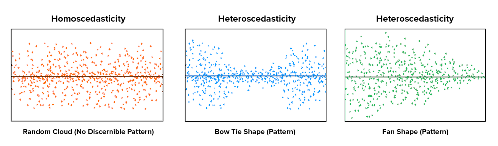
• Constant variance – or homoscedasticity

  

Threats to measurement precision

1. outlier data points

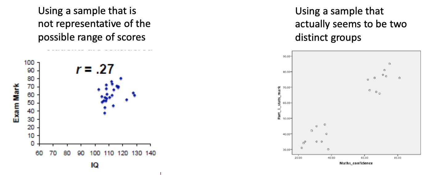
2. range restrictions - limitations in the variability of the data that can lead to biased estimates and reduced statistical power. Understanding these threats is crucial for ensuring the validity of our statistical analyses, as they can significantly impact the reliability of our conclusions.

   • using samples that are not representative of a range of scores

   • using sample that distinctly shows two groups can lead to misleading interpretations, as it fails to account for the full spectrum of data and may ignore important nuances within the population.

Simple Regression

• Correlation to simple regression represents a decision to make one of the variables predict the other variable; this relationship allows us to understand how changes in one variable can affect the other, providing a foundational framework for statistical analysis.

• The predictor goes along the X axes - independent

• The outcome variable is plotted on the Y axes - dependant

• The relationship is the same as independent and dependent variables however the terminology is a bit different ; in simple regression, the independent variable is referred to as the predictor, while the dependent variable is known as the response variable, highlighting their roles in the analysis.

• In this context, it is essential to note that the strength of the relationship can be quantified using the correlation coefficient, which ranges from -1 to 1, indicating the direction and magnitude of the association between the variables.

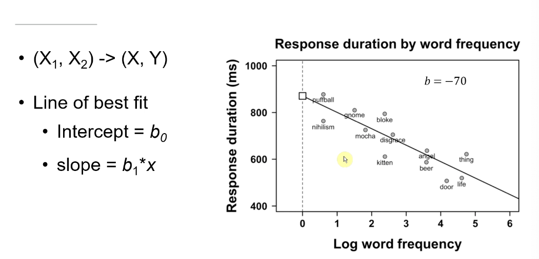
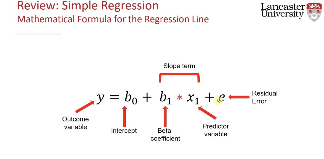
• Regression Line: Composed of an intercept and slope (beta coefficients).

• Mathematical Equation: y = B0 + B1*x + E (where E = error term).

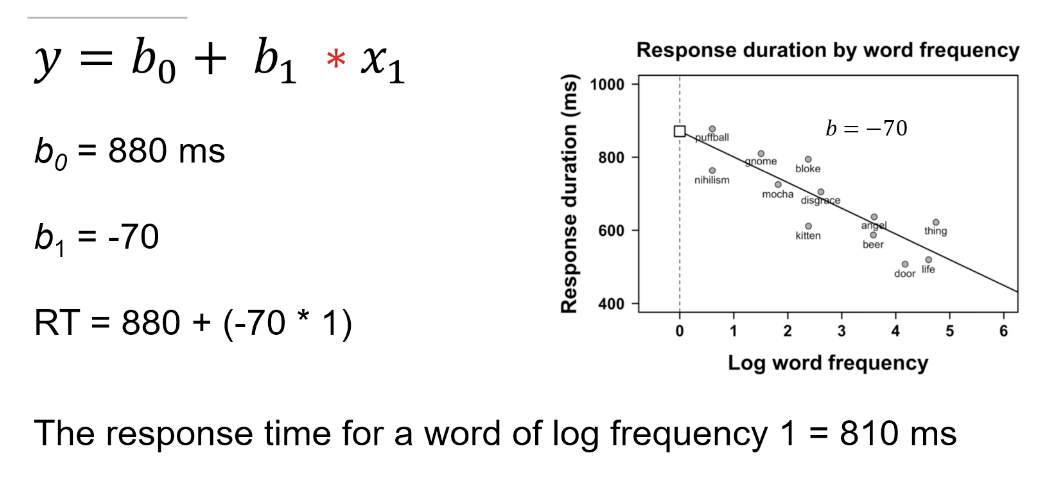
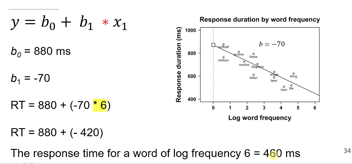
• Predicted values can be generated using the regression model, even for unseen values.

• Line of best fit now known as regression line

• Intercept (B0) - Constant in the model, The intercept represents an average in the outcome variable when continuous predictors are at zero and categorical predictors are at their reference level

• intecpt is like a mean variable r, providing a baseline value that helps to understand the relationship between the predictors and the outcome variable.

• The slope (B1) indicates the change in the outcome variable for each unit increase in the predictor variable, illustrating how the predictors influence the response.

• Measures and represents the model estimation for the best-fitting line for the predictor

• slope helps show the rate of change in y in relation to changes in x, allowing us to quantify the strength and direction of the relationship between the variables.

• as one increases another one decreases by 70 ms , suggesting a strong inverse relationship between the two variables.

• we use the equetaion to help us make predictions

Simple regression assumptions

• include linearity, independence, homoscedasticity, and normality of residuals, which are essential for ensuring the validity of our regression analysis. By adhering to these assumptions, we can better interpret the results and increase the reliability of our predictions.

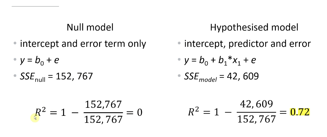
Simple regression - model fit

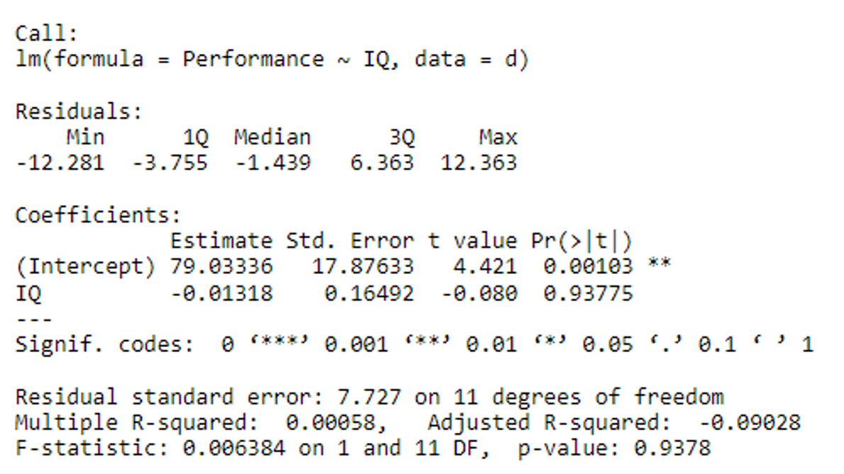
Simple regression - interpreting the output

• Interpretation of Intercept term (b0)

  • Average when all continuous predictors are at 0 or categorical predictors are at their reference level

• Interpretation for continuous coefficients =

• A one unit increase in X gives a change in Y by the amount of

• Interpretation for categorical coefficients =

• A change to another level or group within X gives a change in Y by the amount of b

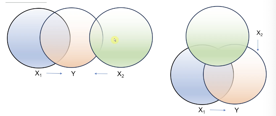
Multiple Regression Insights

• Complexity: Involves multiple predictors but maintains a single intercept; interpretation requires understanding overlapping effects and multicollinearity.

• Model Output: Important to derive coefficients, p-values, and significance levels for each predictor.

• There are more predictor variables

• Some additional work in preparing the dataset for analysis

• Still one intercept

• Some minor differences in interpretation for the intercept

• Still one error term

• Some additional detail for the interpretation and reporting of predictor variables

• Several predictors

  Y = Intercept + predictor 1 + predictor 2 + Error

  Y = b0 + b1 X1 + b2 X2 + e

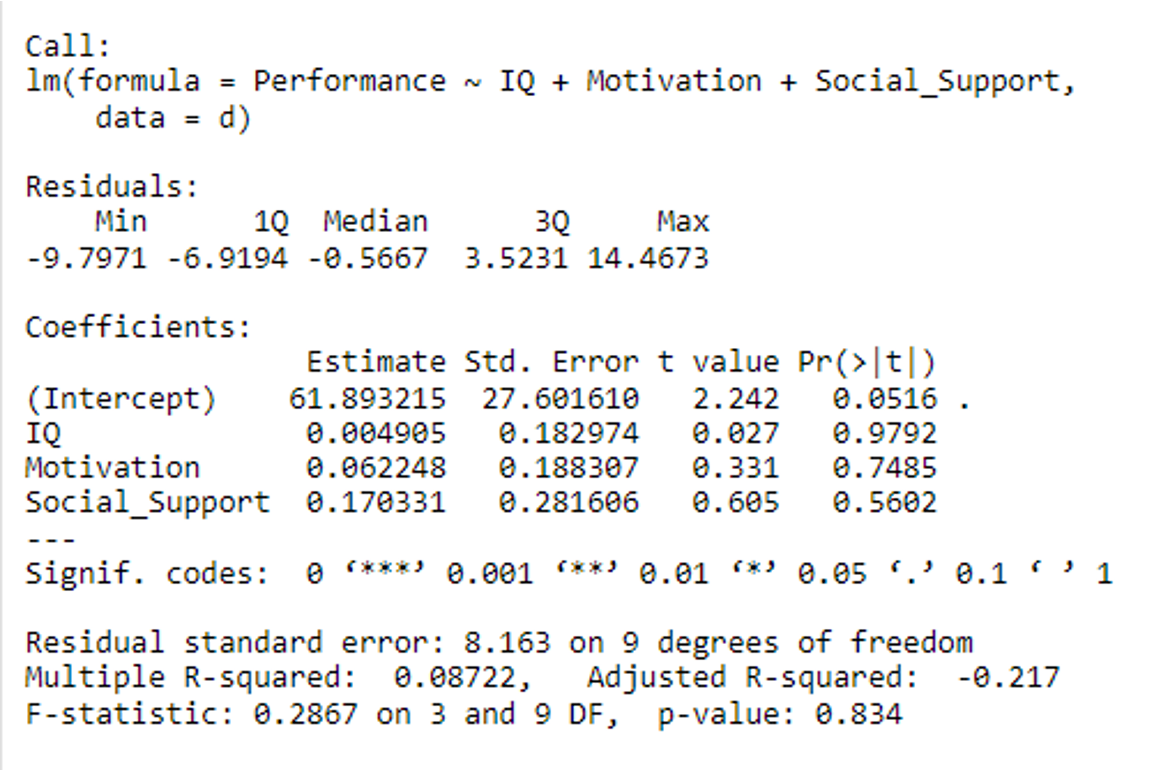
• Interpretation of Intercept term (b0)

  Average when all continuous predictors are at 0 and categorical predictors are at their reference level

• Interpretation for continuous coefficients =

  A one unit increase in X1 gives a change in Y by the amount of b1, when all other predictors are held constant / at their reference level

  A one unit increase in X2 gives a change in Y by the amount of b2, when all other predictors are held constant / at their reference level

Preparedness for Labs

• Recommended Activities: Engage with correlation, simple regression, and multiple regression scripts in R.

• Focus on: Model diagnostics, including residual plots, hat values, and Cook's distance.

Conclusion

• Encourage interactive learning and questions in upcoming labs. Obtain familiarity with regression concepts for success in class test and future research.