Week 11 - Time Series Analysis Notes

Topics

• Autoregressive predictive models

• Statistical inference - the Yule-Walker estimator

• Statistical inference - the OLS estimator

• Nonstationarity

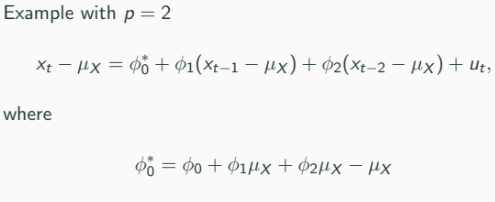
Autoregressive Predictive Models

• Time series prediction often uses autoregressive (AR) models.

  

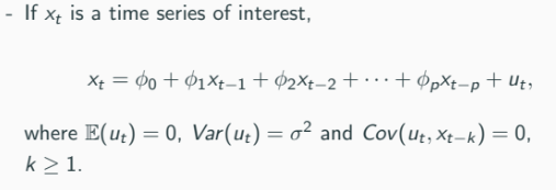
• We use past value to predict the present value.

• Many macroeconomic time series are nonstationary, and methods to deal with this will be considered.

Mean and Variance of a Stationary AR Process

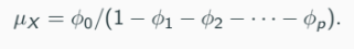
• The mean of a stationary AR(p) process is given by:
  

  

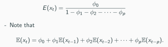
• Strict or weak stationarity implies

  

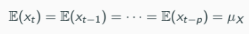
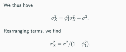
  Thus

  

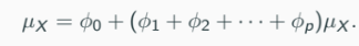
• Rearranging terms, we find:

  

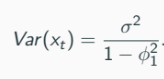
• In the case with p = 1 (assume), the variance of a stationary AR(p) process is given by:

  

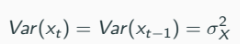
• Note that

  

• (Weak) stationarity implies

  

• An important observation: the variance of Xt is inflated by the persistence ϕ of the AR model.

Autocovariances of a Stationary AR(p) Process

• The autocovariances and autocorrelation functions can be computed by solving the Yule-Walker equations.

  

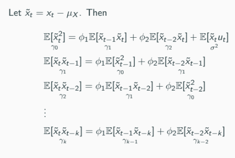
• The Yule-Walker equations (for T = 2, t + 1 and t +2) are given by
  

  

  
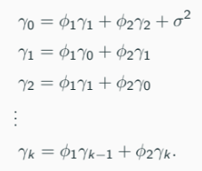
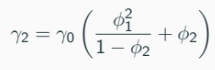
  Autocovariances γ1, …, γk can be computed.

• Suppose that we want to compute γ1 and γ2 (this compute is not the estimate), From the second equation:
  

  

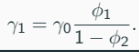
• From the third equation:

  

  
  

  

Statistical Inference - The Yule-Walker Estimator

• Two conventional estimators of (ϕ1, …, ϕp) are

  • Yule-Walker estimator (conventional and widely known)

  • OLS estimator

• In many economic time series, p ≥ 1 seems to be more natural.

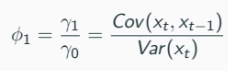
Yule-Walker Estimation: AR(1)

Remember: our coefficients here are the correlation between past and present value.

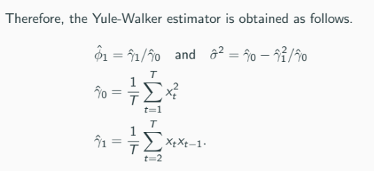
For t = 2, we have t at present and past. For t = 1, only present. ‘t’ in sigma here is basically ‘n’.

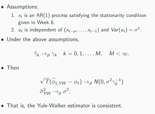
Asymptotic Properties

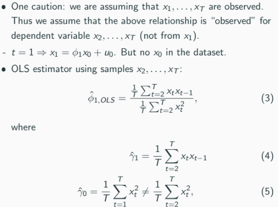
Statistical Inference - The OLS Estimator

OLS Estimation

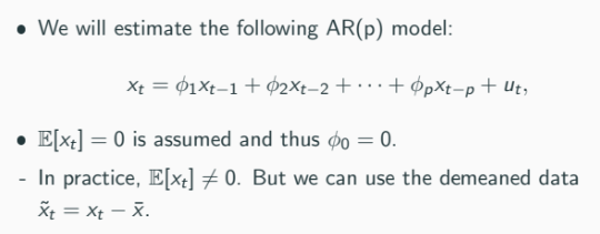
• We will now consider the OLS estimation of
  xt = ϕ₁x_{t-1} + ϕ₂x_{t-2} + ··· + ϕ_px_{t-p} + u_t

• This may be viewed as a linear regression model and x{t-1}, …, x{t-p} may be viewed as regressors.

• It is easy to estimate the above model using OLS. But we will focus on the case p = 1, i.e.,
  xt = ϕ1x{t-1} + ut

• OLS estimation is straightforward.

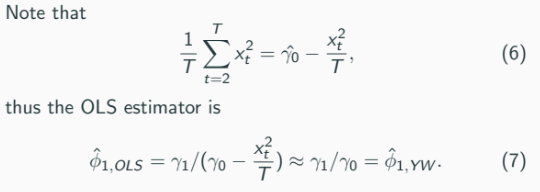
The reason that they are not the same even though the properties of the estimate is very similar, is the account for the ‘time size’.

• OLS accounts for both the ‘time’ size, T = 2, but y₀ only account for 1 ‘time’ size, T = 1. Thus, the OLS might be smaller since we have to account for the correlation between the two past value of OLS compared to the variance only for the YW (covariance of itself = variance).

• In other words: YW only present time autocovariance (when lag is zero, its the variance), it does not explicitly adjust for past value like OLS.

→ Another different between YW and OLS estimates is that OLS depends on the lagging components for its numerator and denominator, hence ‘t’ = 2. Whereas YW uses the variance of itself and doesn’t depend on lagging component (except the numerator), hence the difference in ‘t’.

However, the difference between ϕ̂{1,YW} and ϕ̂{1,OLS} is small if the sample size is large enough.

Asymptotic Equivalence

• Two estimators are not numerically identical (summary of previous point).

  • That is, ϕ̂{YW} ≠ ϕ̂{OLS}.

  • But, |ϕ̂{YW} - ϕ̂{OLS}| →_p 0, i.e., they are asymptotically identical.

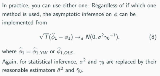
• In practice, you can use either one.

Statistical Inference

• It may be of interest to test
  H0 : ϕ1 = r against H1 : ϕ1 ≠ r

• From the asymptotic results given for the Yule-Walker/OLS estimator ϕ̂1

  

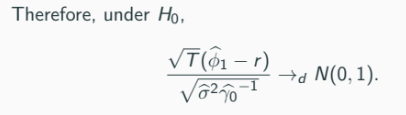
• Confidence interval can be constructed as well.

Forecasting

• Once we estimate the model, the forecasts of future values x{T+1}, x{T+2}, … are given by
  

  

  
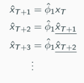
  The forecasts are constructed recursively, as above.

Forecasting (Cont’d)

• Forecasting accuracy measure: when x{T+1}, …, x{T+m} are realized
  

  

  
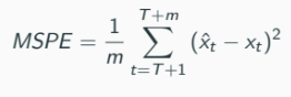
  Forecasting model with smaller MSPE is regarded as better (obviously, smaller variance).

Model with an Intercept

• Suppose that
  xt = ϕ0 + ϕ1x{t-1} + u_t

  • We already know how to estimate this: OLS.

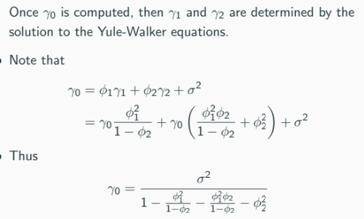
• Alternatively, the Yule-Walker equation tells us that
  

  
  

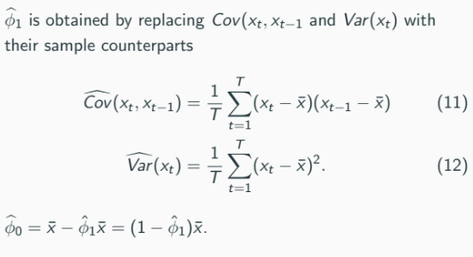
Nonstationarity

• In practice, the use of the AR(p) predictive model may be often problematic since economic time series tends to be nonstationary.

  

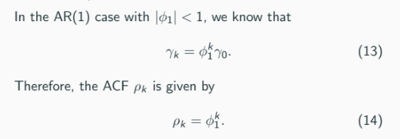
• That is, the ACF ρ_k decays to zero at a fast rate (we proved this in readings of 2150).

  • This is true in a more general case when p > 1.

    

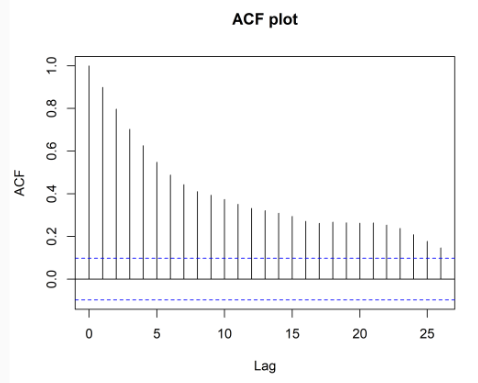
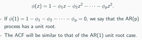
• As shown, the ACF plot time series is not stationary. It is more like the unit root/random walk model, i.e.,
  xt = x{t-1} + u_t

• More generally, in the AR(p) case, the AR(p) equation is characterized by the polynomial
  

  

Differencing

• Such a unit root process can be transformed into a stationary time series by taking differencing (repeatedly if necessary)

  • First-differenced time series: ∆xt = xt - x{t-1}.

  • 

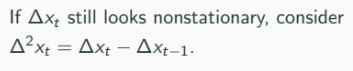
• First-differencing is sufficient for most economic time series.

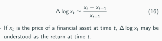
• Sometimes, log-differencing is preferred:

  

AR Predictive Model with Nonstationary Series

• If the considered time series looks nonstationary (check its ACF), we may instead consider ∆xt (or ∆log xt).

• The first differenced time series will be stationary in most cases.

• We then consider the following AR(p) model
  

  

• We may apply the Yule-Walker/OLS estimation methods.