AP Precalculus Unit 2

2.1 - Change in Arithmetic and Geometric Sequences

A sequence is a function from the whole numbers to the real number

Arithmetic Sequences

Geometric Sequences

• Geometric Sequences: Given 2 Terms

  1. Use both terms to create one equation in general form - use the larger k  value term as the g_n term.

  2. Solve for r using the equations from Step 1.

  3. Use the value of r found in Step 2 along with either term given in the problem to write the general form the geometric sequence.

2.2 - Change in Linear and Exponential Functions

Arithmetic Sequences and Linear Functions

Geometric Sequences and Exponential Functions

Linear Functions vs. Exponential Functions

2.3 - Exponential Functions

Key Characteristic of Exponential Functions

An exponential function has the general form f\left(x\right)=a\left(b\right)^{x} , b>0 where a and b are constants with a\ne0 and b\ne1	a represents the initial amounts. b represents the common ratio
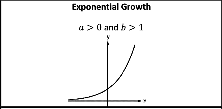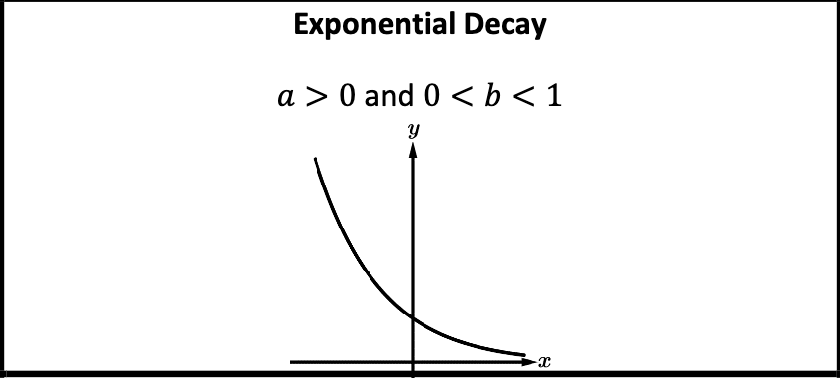Exponential functions are always increasing or always decreasing. They will never switch from one to the other, so they have no relative extrema	Exponential functions are always concave up or always concave down. They will never switch concavity, so they have no points of inflection.
For exponential functions in general form, as the input values increase/decrease without bound, the output values will increase/decrease without bound or they will approach zero.	\lim_{x\to\pm\infty}ab^{x}=\infty or \lim_{x\to\pm\infty}ab^{x}=-\infty or \lim_{x\to\pm\infty}ab^{x}=0

2.4 - Exponential Function Manipulation

• Exponent Rules

  • Product Property: b^{m}b^{n}=b^{m+n}

  • Power Property: \left(b^{m}\right)^{n}=b^{mn}

  • Negative Exponent Property: b^{-n}=\frac{1}{b^{n}}

• Transformations

  • Horizontal translation - g\left(x\right)=2^{\left(x+3\right)}

  • Vertical dilation - g\left(x\right)=8\left(2\right)^{x}

  • Horizontal dilation - g\left(x\right)=2^{\left(3x\right)}

  • Vertical translation - g\left(x\right)=2^{x}+3

  • Change in base - g\left(x\right)=8^{x}

2.5 - Exponential Function Context and Data Modeling

• Modeling Exponential Functions from Data

  • An exponential function can be constructed if given either

    1. The common ratio and the initial value, or

    2. Two input-output pairs

• The Natural Base: e

• Percent Increase:

  • Start with the the initial amount “a” and grow with % increase

  • y=a\left(l+r\right)^{x}

• Percent Decrease:

  • Start with the the initial amount “a” and grow with % increase

  • y=a\left(l-r\right)^{x}

• Half-Life:

  • An initial amount a that shrink by half every h

  • f\left(t\right)=a\left(\frac12\right)^{\frac{t}{h}}

• Doubling time:

  • An initial amount a that doubles every d

  • f\left(t\right)=a\left(2\right)^{\frac{t}{d}}

2.6 - Competing Function Model Validation

Comparing Linear, Quadratic, and Exponential Models

Type of Model	Example Graph	Example Data Table	Important Features
Linear		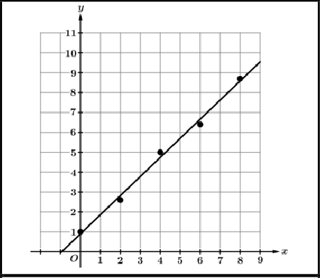	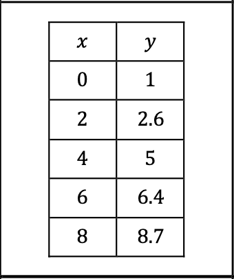Use a linear model when the data reveals a relatively constant rate of change.
Quadratic		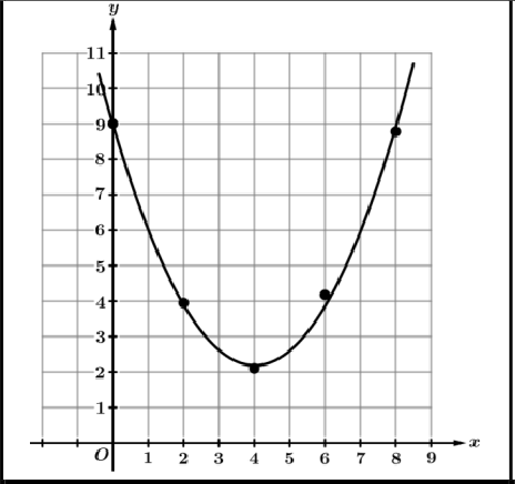	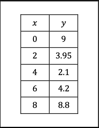Use a quadratic model when the rates of change are increasing/decreasing at a relatively constant rate
Exponential		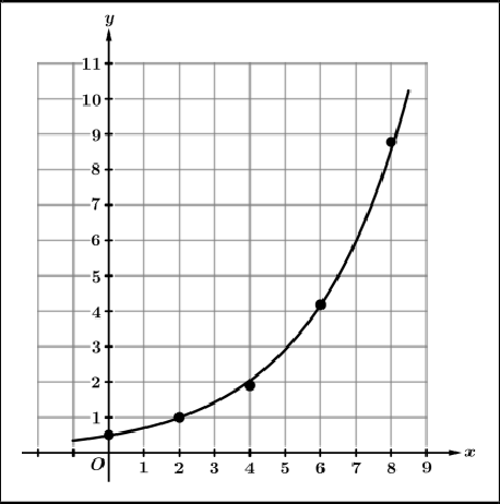	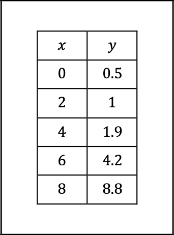Use an exponential model when the output values are roughly proportional. Each successive output is approximately the result of repeated multiplication.

Residuals

• When creating a model, you can use your model to predict values for the dependent variable given an independent variable

  • When using a model, it is important to remember this is only a PREDICTED value.

  • Residual = Actual Output Value - Predicted Output Value

Using a Residual Plot to Check the Appropriateness of a Model

• If a model for a given set of data is appropriate, the residual plot should appear without a pattern.

2.7 - Compositions of Functions

• Composite Functions

  • There are 2 ways to write composite functions:

  • f\left(g\left(x\right)\right) or fog\left(x\right)

  • These are read as f of g of x

    • When working with composite functions, starts on the inside

• Domain of a Composed Function

  • Two find the domain of a composed function f\left(g\left(x\right)\right) , there are two restrictions to consider

    1. Since g(x) is the input, only use x-values that are in the domain of g.

    2. The output of g(x) must be in the domain of f(x), any restrictions on the domain f\left(g\left(x\right)\right) must also be included

• Decomposition of Functions

  • Functions given analytically can often be decomposed into complex functions

2.8 - Inverse Functions

An inverse relation will “undo” a given relation. Every inverse relation can be found by switching each x and y value.

•     Numerical (Tables)

  • Switch the x and y values to find the inverse

An inverse will not be a function if there is more than 1 x values/not a 1:1 ratio.

• Graphical (Pictures)

  • Take the value of each point, switch the x and y value and plot the new point

The graphs of inverse are reflected over the line y=x

• Analytical (Equations)

  • To Find an Inverse Equation:

    • Switch the x and y values

    • Solve for y (Get y by itself)

The inverse function of f\left(x\right) is written as f^{-1}\left(x\right)

• Finding Inverse Functions of Rational Functions (with multiple x’s)

  1. Switch the x and y values

  2. Multiply/Distribute both sides by the denominator of the rational expression to eliminate the fraction.

  3. Move all terms that include the variable y to the left side of the equation and move all terms that do not include the variable y to the right side of the equation.

  4. Factor out a y from the terms on the left side of the equation.

  5. Divided both sides by the terms remaining on the left side after y was factored out.

  6. Rewrite the equation with proper inverse notation (f^{-1}\left(x\right))

• Sketching an Inverse Graph

  1. Sketch the line y = x on the graph

  2. Mark any points from the original graph that are already on the line. These points stay the same

  3. Select a few additional points on the original graph and find their inverse points

  4. Sketch the inverse graph by connecting the new points in a similar pattern to the original function.

• Inverse Functions

  • Two functions f(x) and g(x) are inverses if and only if f(g(x)) = x and g(f(x)) = x, must show that both of these functions equal x

  • With inverse functions the domain of f is the range off^{-1}

  • If a function changes from increase to decreasing (or vice versa), it will not pass the horizontal line test and therefore its inverse relation will not pass the vertical line test as a result.

2.9 - Logarithmic Expressions

Every operation has exactly one inverse operation

Exponentials can be rewritten in logarithm from

• If the base of a log expression is 10, it is called common log and is written without a base

• Log expressions can sometimes be evaluated without the use of a calculator by using the equivalent exponential form.

2.10 - Inverses of Exponential Functions

• General Form of a Logarithmic Functions

  • f\left(x\right)=a\log_{b}x where b>0,b\ne1, and a\ne0

Because exponential functions and logarithmic functions are inverses of each other, the characteristics of the input-output values of an exponential function will become the characteristics of the output-input values of a logarithmic function.

• Exponential and Logarithmic Tables

  • Exponential Functions: over equal-width input-value intervals, the output values change multiplicatively.

  • Logarithmic Functions: over equal-width output values, the input values are changing multiplicatively.

• Exponential and Logarithmic Functions as Inverses

  • If f\left(x\right)=b^{x} and g\left(x\right)=\log_{b}x , the f and g are inverse functions

2.11 - Logarithmic Functions

Key Characteristics of Logarithmic Functions

• General Form

  • f\left(x\right)=a\log_{b}x , b>0

    • where a and b are constants with a\ne0 and b\ne1

  • Domain: \left(0,\infty\right)

  • Range: \left(-\infty,\infty\right)

a>0 and b>1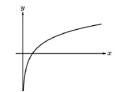

a<0 and b>1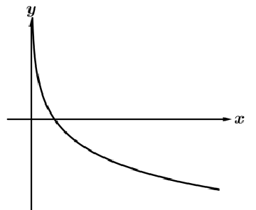

• Increasing vs. Decreasing

  • Logarithmic functions are always increasing or always decreasing.

    • They have no relative extrema.

• Concave Up vs. Concave Down

  • Logarithmic functions are alway concave up or always concave down.

    • They have no points of inflections

• End Behavior

  • in general form, as the input values increase without bound, the output values will increase/decrease without bound.

  • Since logarithmic functions have a restricted domain, they have a vertical asymptote at x = 0. So the left end behavior will be x → 0^{+} .

• Limit Statements

  • \lim_{x\to0^{+}}a\log_{b}x=\pm\infty

  • \lim_{x\to+\infty}a\log_{b}x=\pm\infty

2.12 - Logarithmic Functions Manipulation

• Properties of Logarithms

  • Product Property

    • \log_{b}\left(xy\right)=\log_{b}x+\log_{b}y

  • Quotient Property

    • \log_{b}\left(\frac{x}{y}\right)=\log_{b}x-\log_{b}y

  • Power Property

    • \log_{b}x^{n}=n\log_{b}x

  • Change of Base

    • \log_{b}x=\frac{\log_{a}x}{\log_{a}b} where a>0 and a\ne1

• The Natural Log Function

  • \log_{e}x=\ln x

• Finding Inverses of Logarithmic and Exponential Functions

  1. Switch the roles of x and y in the equation

  2. Use inverse operations to solve for y in the inverse relation

  3. Write the final inverse function using proper notation.

2.13 - Exponential and Logarithmic Equations and Inequalities

• Properties of Exponents

  • Product Property

    • b^{m}b^{n}=b^{m+n}

  • Power Property

    • \left(b^{m}\right)^{n}=b^{mn}

  • Negative Exponent Property

    • b^{-n}=\frac{1}{b^{n}}

• Properties of Logarithms

  • Product Property

    • \log_{b}\left(xy\right)=\log_{b}x+\log_{b}y

  • Quotient Property

    • \log_{b}\left(\frac{x}{y}\right)=\log_{b}x-\log_{b}y

  • Power Property

    • \log_{b}x^{n}=n\log_{b}x

• Converting Between Exponential and Logarithmic Form

  • Exponential Form: a=b^{c} \lrArr Logarithmic Form: \log_{b}a=c

• Solving Exponential and Log Equations Involving Only 1 Logarithm or Exponent

  1. Isolate the exponential or log expressions on one side of the equation

  2. Convert the equation to the alternate form

  3. Solve for any variable

  4. Simplify and/or round answer

• Equations with Multiple Logarithms

  • Simplify to either form and solve accordingly

    • Form 1 - \log_{a}\left(x\right)=b

      • Finish solving by converting to exponential form

    • Form 2 - \log_{a}\left(x\right)=\log_{a}\left(y\right)

      • Finish solving by setting x = y

  • CHECK FOR EXTRANEOUS SOLUTIONS

  • Do not just cancel logs, simplify

• Equations with Multiple Exponentials

  • Find common bases using properties of exponents

• Solving Inequalities Involving Logarithmic and Exponential Functions

  • Solve the same way as inequalities of polynomial and rational functions

2.14 - Logarithmic Function Context and Data Modeling

• Logarithmic Function Models

  • y=a+b\ln x or y=a+b\log x where a and b are constants and b\ne0

2.15 - Semi - log Plots

a semi - log plot will have one axis logarithmically scaled, exponential functions will appear linear

• Linear Models for a Semi - log Plot

  • given the model , the corresponding linear model for a semi - log plot is: y=\left(\log_{n}b\right)x+\log_{n}a

  • where n>0 and n\ne1

  • The slope of the linear function is \log_{n}b and the y-intercept is \log_{n}a

  • The base n corresponds to the base used for the scaling of the vertical axis