Chapter 8 - Consumption, Saving, Investment, and the Multiplier

8.1 Consumption and Saving

Consumption and Savings Functions

• Disposable income (DI) - The income a consumer has left over to spend or save once they have paid out net taxes.

  

  • Net taxes = Taxes paid - Transfers received.

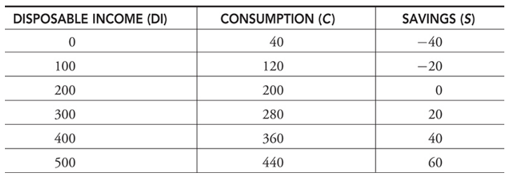
Consumption and Saving Schedules

• Consumption and saving schedules - Tables that show the direct relationships between disposable income and consumption and saving. As DI increases for a typical household, C and S both increase.

  

Consumption

• Consumption function - A linear relationship showing how increases in disposable income cause increases in consumption.

  

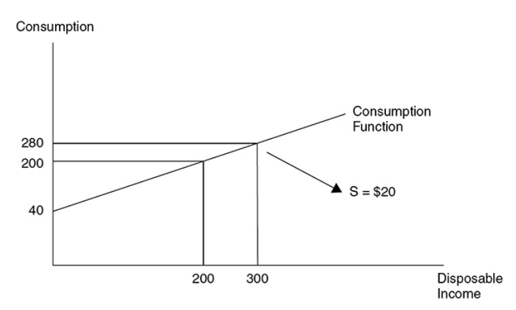
• C = 40 + .80(DI)

• The constant $40 is referred to as autonomous consumption because it does not change as DI changes. The slope of the consumption function is .80.

• Autonomous consumption - The amount of consumption that occurs no matter the level of disposable income. In a linear consumption function, this shows up as a constant and graphically it appears as the y-intercept.

• Dissaving - Another way of saying that saving is less than zero. This can occur at low levels of disposable income when the consumer must liquidate assets or borrow to maintain consumption.

• Saving function - A linear relationship showing how increases in disposable income cause increases in saving.

  

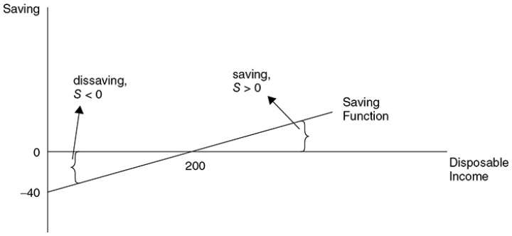
• S = -40 + .20(DI)

• The constant $–40 is referred to as autonomous saving because it does not change as DI changes. With zero disposable income, the household would need to borrow $40 to consume $40 worth of goods. The slope of the saving function is .20.

• Autonomous saving - The amount of saving that occurs no matter the level of disposable income. In a linear saving function, this shows up as a constant, and graphically it appears as the y-intercept.

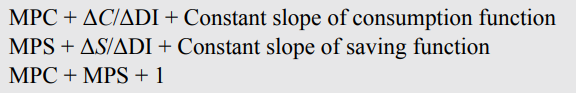
Marginal Propensity to Consume and Save

• Marginal propensity to consume (MPC) - The change in consumption caused by a change in disposable income, or the slope of the consumption function.

  

• ^^Ex. →^^ In the first table, we see that for every additional $100 of DI, C increases by $80, so the MPC + .80.

• Marginal propensity to save (MPS) - The change in saving caused by a change in disposable income, or the slope of the saving function.

  

• ^^Ex. →^^ Using the first table, we can see that for every additional $100 of DI, S increases by $20, so the MPS + .20.

• For every additional dollar not consumed, it is saved. So if the consumer gains $100 in disposable income, they increase their consumption by $80 and increase saving by $20. In other words, MPC + MPS + 1.

  

Changes in Consumption and Saving

• A change in disposable income causes a movement along the consumption and savings functions.

Determinants of Consumption and Saving

• Determinants of consumption and saving - Factors that shift the consumption and saving functions in the opposite direction are wealth, expectations, and household debt. The factors that change consumption and saving functions in the same direction are taxes and transfers.

  • Wealth - When the value of accumulated wealth increases, consumption functions shift upward, and the saving function shifts downward, because households can sell stock or other assets to consume more goods at their current level of disposable income.
  • Expectations - Uncertainty or a low expectation about future income usually prompts a household to decrease consumption and increase saving. An expectation of a higher future price level spurs higher consumption right now and less saving.
  • Household debt - Households can increase consumption with borrowing, or debt. However, as households accumulate more and more debt, they need to use more and more disposable income to pay off the debt and thus decrease consumption.
  • Taxes and transfers - If the government increases taxes, households see both consumption and saving decrease because more of their gross income is sent to the government. On the other hand, an increase in government transfer payments increases both consumption and saving functions. In the case of taxes and transfers, consumption and saving functions shift in the same way.

• An upward shift in consumption tells us that at all levels of disposable income, consumption is greater. If consumption is greater at all levels of disposable income, saving must be lower and vice versa.

  • The only exception is the case of taxes and transfers.

  

  

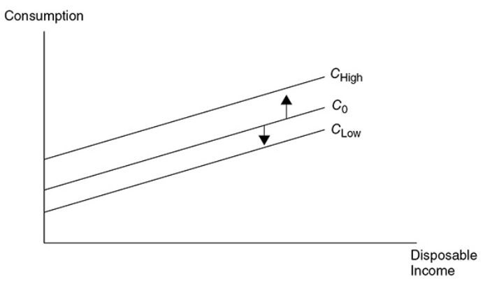
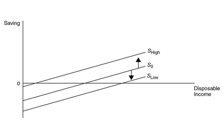
Exceptions in the graph

• In the exception of taxes and transfers, when the consumption function shifts upward, the saving function shifts downward.
• In the exception of taxes and transfers, when the consumption function shifts downward, the saving function shifts upward.
• When taxes increase (or transfers decrease), both consumption and saving functions shift downward.
• When taxes decrease (or transfers increase), both consumption and saving functions shift upward.

8.2 Investment

Decision to Invest

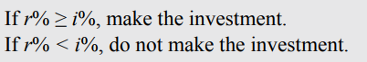
• Decision to invest - This decision is based on marginal benefits and marginal costs. A firm invests in projects as long as r ≥ i.
  • The marginal cost of the investment - The real rate of interest (i), or the cost of borrowing.
• Expected real rate of return (r) - The rate of real profit the firm anticipates receiving on investment expenditures. This is the marginal benefit of an investment project.
  • ^^Ex. →^^ A local pizza firm invests $10,000 in a new delivery car. The owner expects this to help to deliver more pizzas, increasing revenues and profits. The car lasts exactly one year, and increased real profits are anticipated to be $2,000. This expected real rate of return is $2,000/$10,000 = .20 or 20%.
• Real rate of interest (i) - The cost of borrowing to fund an investment. This can be thought of as the marginal cost of an investment project.
  • ^^Ex. →^^ The owner goes to the bank and asks for a one-year loan to purchase the new delivery car. The bank offers a nominal rate of interest of 15 percent; this includes 5 percent for expected inflation and 10 percent as the real rate of borrowing the money for a year. At the end of the year, the owner spends $1,000 as real interest on the $10,000 loan.

The Decision

• Since the new delivery car provides $2,000 in additional real profits (r + 20%), and the loan costs $1,000 in real interest (i + 10%), this investment should be made.

  

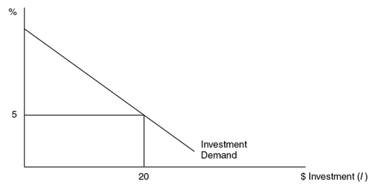
Investment Demand

• Investment demand - The inverse relationship between the real interest rate and the cumulative dollars invested. Like any demand curve, this is drawn with a negative slope.

• Investment demand curve - Shows the inverse relationship between the interest rate and the cumulative dollars invested.

  

Investment and GDP

• In the simple model of private investment, there is no GDP or disposable income. With no government or foreign sector, GDP + DI. We assume that investment spending (I) is determined from the investment demand curve and is constant at all levels of GDP.

• Autonomous investment - The level of investment determined by investment demand. It is autonomous because it is assumed to be constant at all levels of GDP.

  

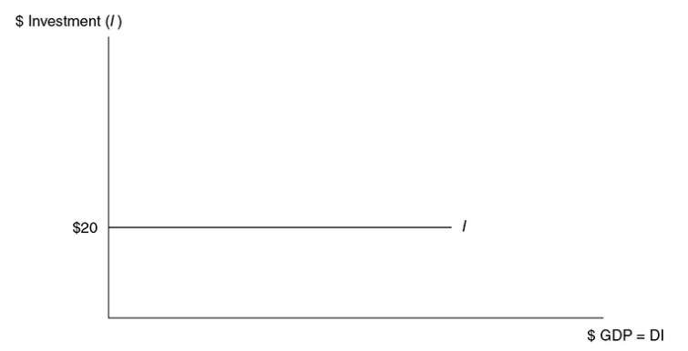
• ^^Ex. →^^ In the previous graph, if the interest rate was 5%, firms would invest $20 billion this year, regardless of the level of disposable income or GDP. This autonomous investment is illustrated in the second graph as a horizontal line with GDP on the x-axis. If something happened to interest rates, or to investment demand, autonomous investment could increase or decrease but, at that new level, would be constant at any value of GDP.

Market for Loanable Funds

• Market for loanable funds - The market for dollars that are available to be borrowed for investment projects. Equilibrium in this market is determined at the real interest rate where the dollars saved (supply) is equal to the dollars borrowed (demand).

Demand for Loanable Funds

• Demand for loanable funds - The negative relationship between the real interest rate and the dollars invested and borrowed by firms and by the government.

Supply of Loanable Funds

• Supply of loanable funds - The positive relationship between the dollars saved and the real interest rate.

• Private saving - Saving conducted by households and equal to the difference between disposable income and consumption.

  

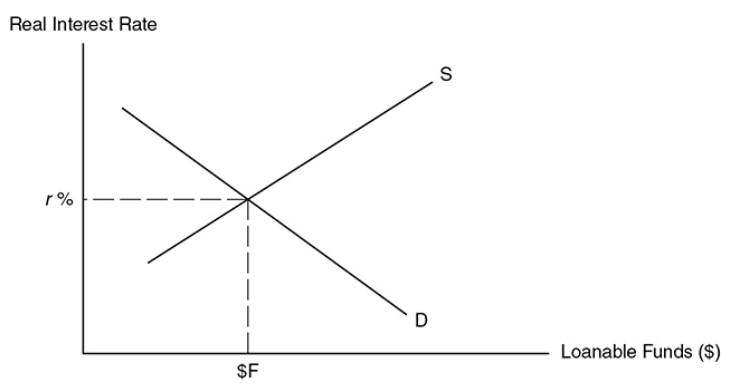
• This is the market for loanable funds and the equilibrium interest rate is found at the intersection of the supply and demand curves.

  • The supply of loanable funds comes from saving and lending.
  • The demand for loanable funds comes from investment and borrowing.
  • Equilibrium is at the real interest rate where dollars saved equals dollars invested.

8.3 The Multiplier Effect

• Multiplier effect - Describes how a change in any component of aggregate expenditures creates a larger change in GDP.

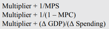
• Spending multiplier

  

Public and Foreign Sectors

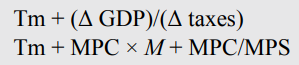
Tax multiplier

• Tax multiplier - The magnitude of the effect that a change in taxes has on real GDP.

  

• ^^Ex. →^^ The MPC is equal to .90, and the government transfers back tax revenue to consumers by sending each taxpayer a $200 check. With an MPC = .90, $180 is consumed and $20 is saved. The multiplier process kicks in, but not on the entire $200, only on the consumed portion of $180. The multiplier being 1/.10 + 10, GDP increases by $1,800. In other words, a $200 change in tax policy (a tax rebate in this case) caused a $1,800 change in real GDP.

The difference in multipliers

• With an MPC = .90, the spending multiplier is 10, but the tax multiplier is smaller, Tm + 9. Why? The spending multiplier begins to work as soon as there is a change in autonomous spending (C, I, G, net exports), but the tax multiplier must first go through a person’s consumption function as disposable income.

Balanced-budget multiplier

• Balanced-budget multiplier - When a change in government spending is offset by a change in lump-sum taxes, real GDP changes by the amount of the change in G; the balanced-budget multiplier is thus equal to 1.
  • ^^Ex. →^^The government wants to spend $100 on a federal program and pay for it by collecting $100 in additional taxes. The MPC = .90 in this example.
  • The spending multiplier + 10 implies that the $100 of new spending (G) creates a $1,000 increase in real GDP.
  • The tax multiplier Tm + 9 implies that a $100 increase in taxes decreases real GDP by $900.
  • Change in real GDP + $1,000 – $900 + $100
  • So a $100 increase in spending, financed by a $100 increase in taxes, created only $100 in new GDP. The balanced-budget multiplier is always equal to 1, regardless of the MPC.