AP Statistics - Chapter 7
7.1
Population - total group being focus on
- Parameter - proportion of population
Sample - group out of population being evaluated
- Statistic - proportion of sample
| mean | proportion | standard deviation | |
|---|---|---|---|
| parameter | µ | p | σ |
| statistic | x̄ | p̂ | s |
A statistic is an unbiased estimator of a parameter if the sampling distribution mean is equal to the parameter
An increase in sample size decreases variability
7.2
Evaluating a Claim:
- Assume it’s true
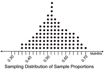
- Created a simulated sampling distribution
- Find the percent chance of getting observed result and evaluate
If a sample occurs that is less than 5% of the sampling distribution, then there is convincing evidence to disprove a claim, if it is greater than 5%, there is not convincing evidence
7.3
10% Condition (checks for independence): if a sample is less than or equal to 10% of a population, independence can be assumed
Large Counts Condition (checks for normality): if np≥10 and n(1-p)≥10, then the distribution is approximately normal
µ(p̂) = p
σ(p̂) = √((p(1-p))/n)
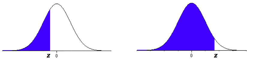
z = (p̂-µ(p̂))/(σ(p̂))
7.4
Two Sample Distributions (two samples being combined into one sampling distribution)
µ(p̂1-p̂2) = p1-p2
σ(p̂1-p̂2) = √((p1(1-p1))/n1+(p2(1-p2))/n2)
z = ((p̂1-p̂2)-µ(p̂1-p̂2))/(σ(p̂1-p̂2))
7.5
µ(x̄) = µ
σ(x̄) = σ/√(n)
z = (x̄-µ(x̄))/(σ(x̄))
If the shape of a population is approximately normal, then the shape of the sampling distribution is approximately normal.
7.6
Central Limit Theorem: a sampling distribution is approximately normal is n≥30
7.7
Two Sample Distributions (two samples being combined into one sampling distribution)
µ(x̄1-x̄2) = µ(x̄1) - µ(x̄2) = µ(1) - µ(2)
σ(x̄1-x̄2) = √((σ1^2)/n1 + (σ2^2)/n2)
z = ((x̄1-x̄2)-µ(x̄1-x̄2))/(σ(x̄1-x̄2))