1. Sensitivity Analysis

Page 1: Introduction to What-if Analysis

• Topic: What-if Analysis (Sensitivity Analysis) for Linear Programming

• Instructor: Rim Jaber

• Course: ADM2302

Page 2: Understanding the Assumptions

• Assumption: Model parameters are known with certainty.

• Reality: Model parameters are estimates and can change.

• Example: Referring to the RMC Problem for context.

Page 3: The RMC Example

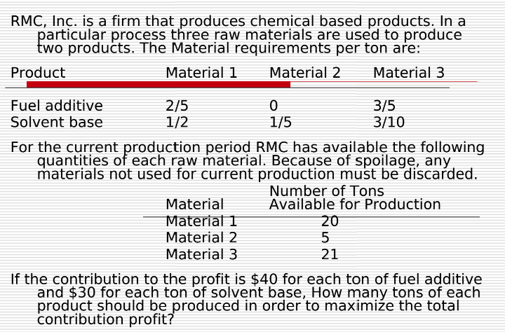
• Company Overview: RMC, Inc. produces chemical-based products using three raw materials for two products.

• Material Usage per Product:

  • Fuel Additive:

    • Material 1: 2/5 tons per ton

    • Material 2: 0 tons

    • Material 3: 3/5 tons per ton

  • Solvent Base:

    • Material 1: 1/2 tons per ton

    • Material 2: 1/5 tons per ton

    • Material 3: 3/10 tons per ton

• Available Material for Production:

  • Material 1: 20 tons

  • Material 2: 5 tons

  • Material 3: 21 tons

• Profit Contribution:

  • Fuel Additive Profit: $40/ton

  • Solvent Base Profit: $30/ton

• Goal: Determine tons of each product to maximize total profit.

Solution:

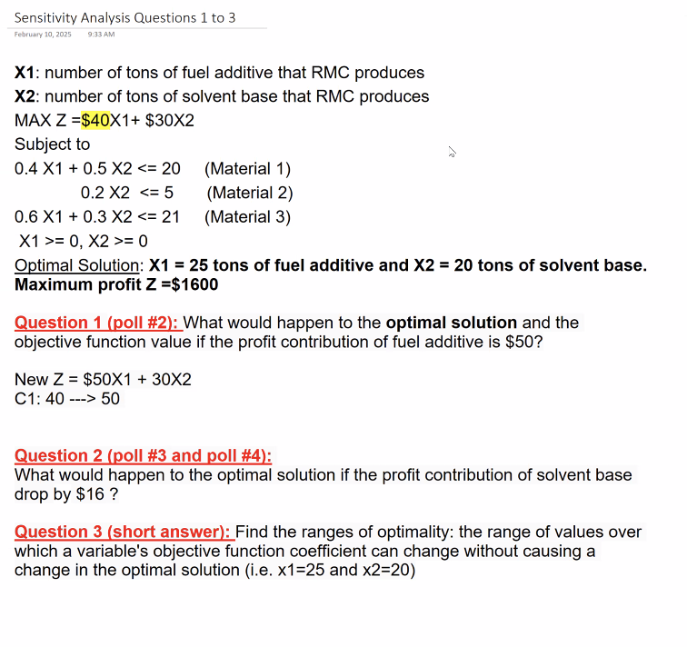
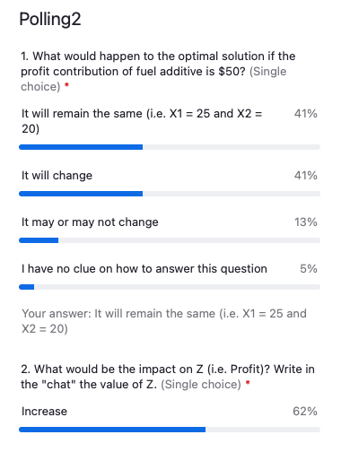
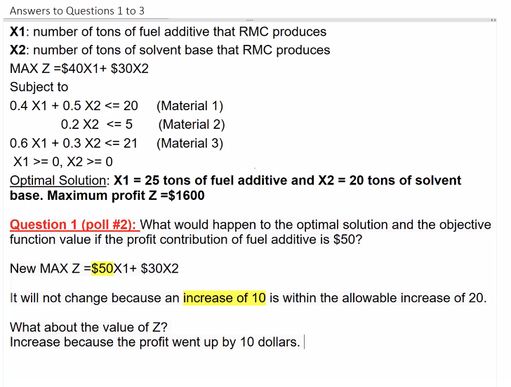
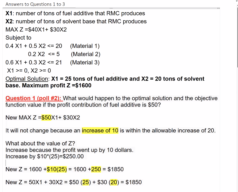
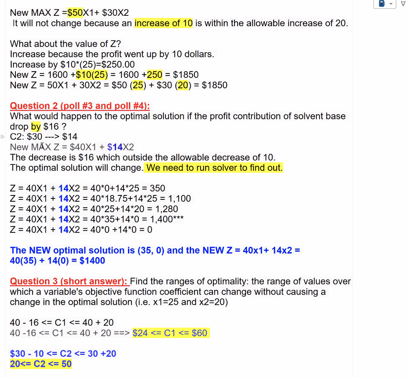
• it will remain the same because between $40 and $50 there is a change of 10 which is allowable because it is within the allowable increase of 20 (0.4X1+0.5X2<=20)

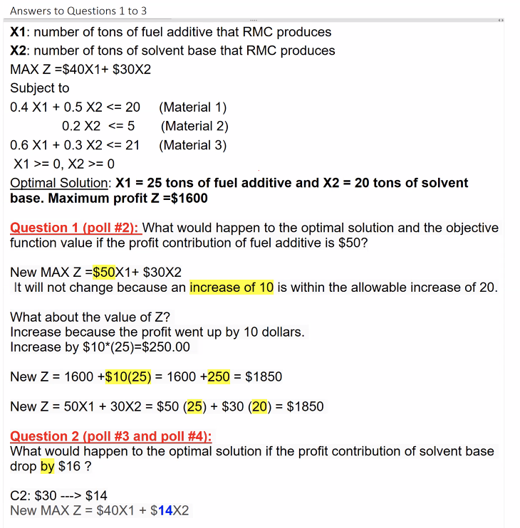
• The new optimal solution would now be (35,0) because the profit contribution of solvent based has dropped (Q2)

  

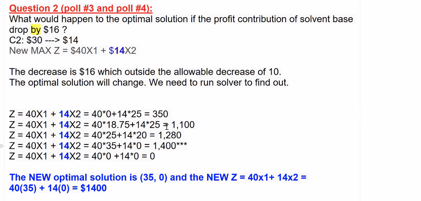
• if we change binding constraints then the corner points would change

Page 4: Formulation of RMC Problem

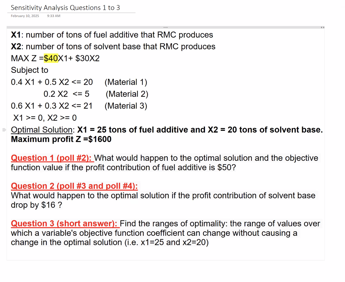
• Objective Function:

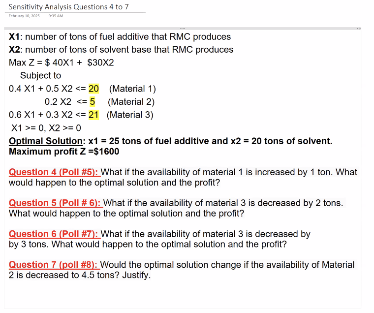
  • Maximize Z = $40 * x1 + $30 * x2

• Constraints:

  • (2/5)x1 + (1/2)x2 ≤ 20 (Material 1)

  • (1/5)x2 ≤ 5 (Material 2)

  • (3/5)x1 + (3/10)x2 ≤ 21 (Material 3)

  • x1 ≥ 0, x2 ≥ 0

• Variables:

  • x1: tons of fuel additive

  • x2: tons of solvent base

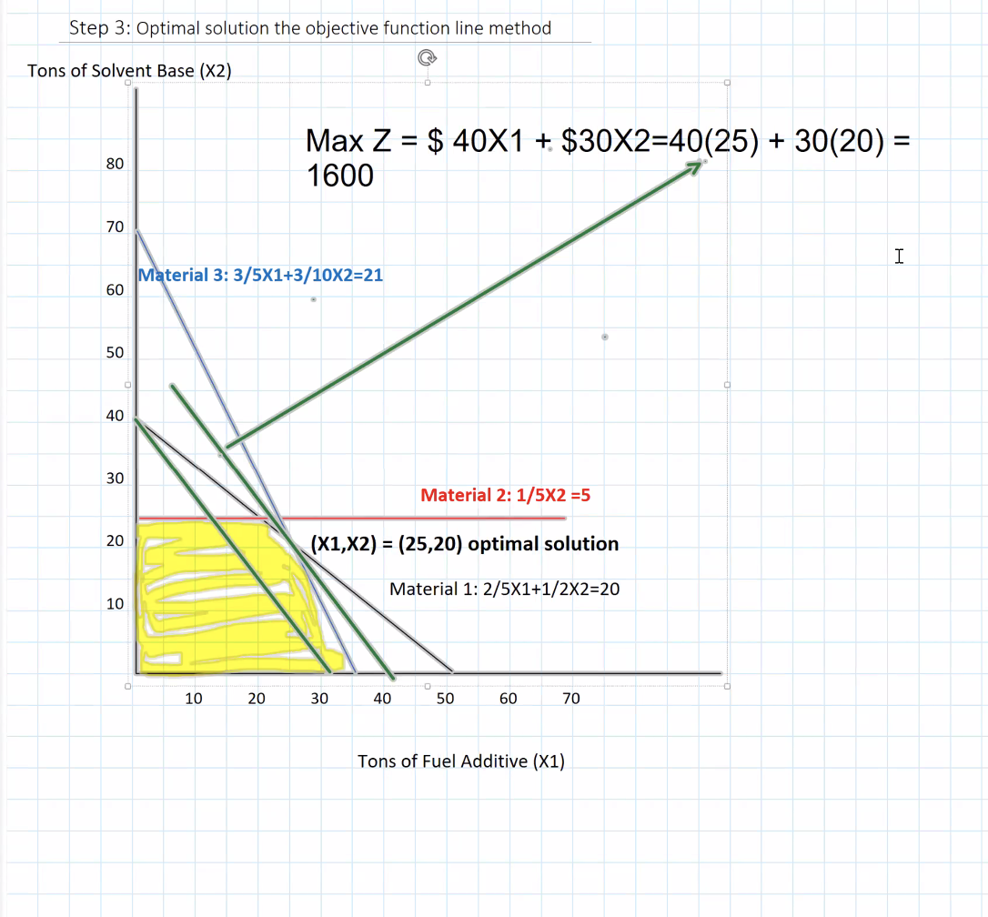
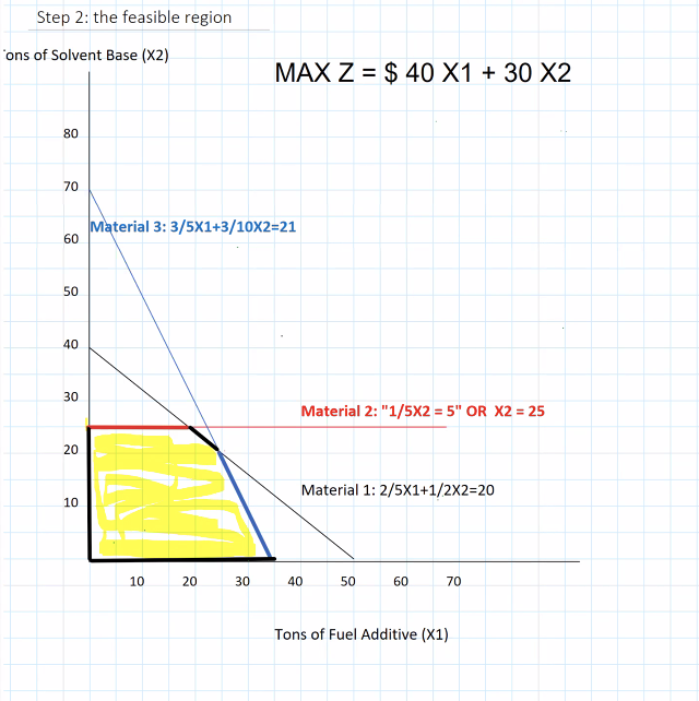
Page 5: The Feasible Region

• Graph:

  • x1 on horizontal axis

  • x2 on vertical axis

• Constraints represented as lines:

  • 2/5x1 + 1/2x2 = 20

  • 1/5x2 = 5

  • 3/5x1 + 3/10x2 = 21

Page 6: Finding Optimal Solution

• Corner Points Identified:

  • (25, 20), (18.75, 25), (0, 25), (0, 0), (35, 0)

• Optimal Solution using Corner Point Method:

  • Calculation of Z for each point

Page 7: Optimal Solution Analysis

• Calculated Values of Z:

  • Z(25, 20) = $750

  • Z(18.75, 25) = $1500

  • Z(0, 25) = $0

  • Z(35, 0) = $1400

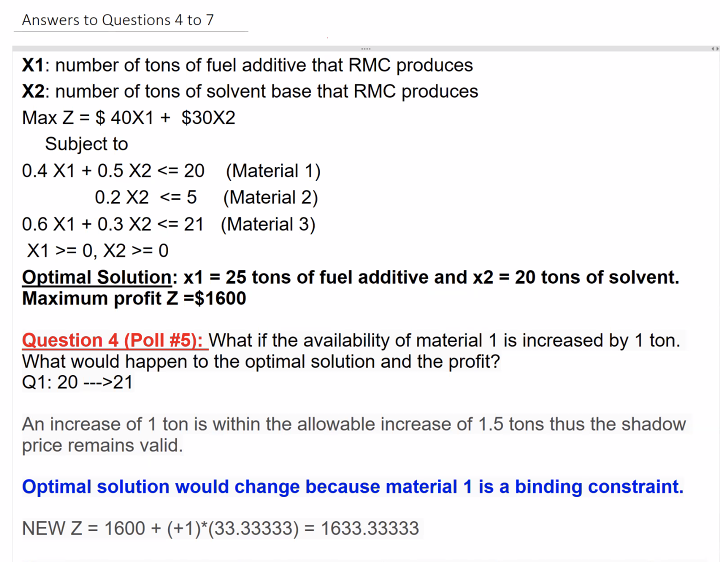
  • Z(25, 20) = $1600

• Optimal Solution Found: at (25, 20)

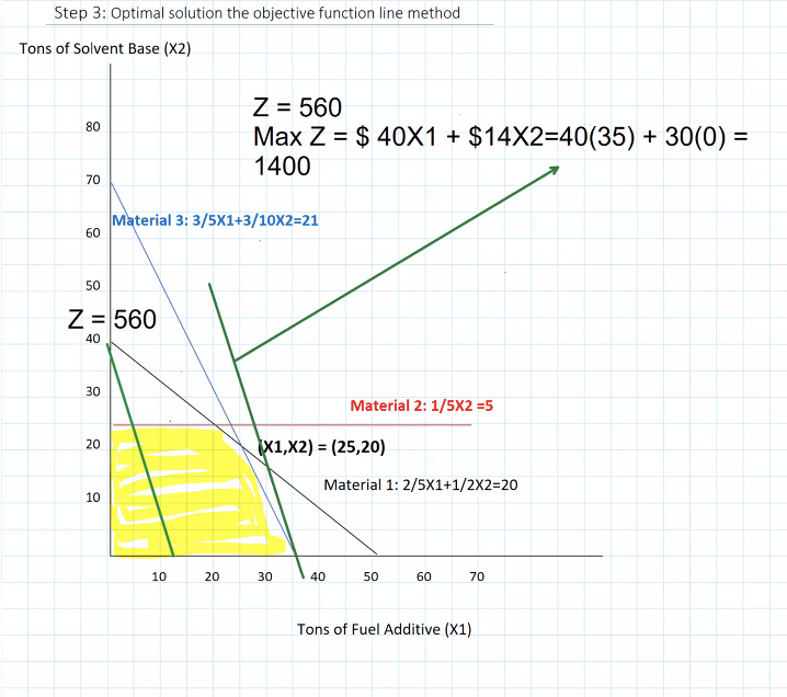
Page 8: Objective Function Line Method

• Maximum Isoprofit Line:

  • Represented as Z = $1600

  • Optimal Solution Point identified at (25, 20)

Page 9: Developing a Spreadsheet Model

• Spreadsheet Reference: RMC_Problem.xlsx

• Formula Examples:

  • fx =SUMPRODUCT(B5:C5,$B$3:$C$3)

• Variables in Spreadsheet:

  • D5: Solution

  • D8 to D10: Material constraints analyzed

Page 10: Objective Cell Summary

• Profit Totals:

  • Original: $0

  • Final Value: $1,600

• Variable Cells:

  • x1 (Fuel Additive): 0 to 25

  • x2 (Solvent Base): 0 to 20

• Binding Constraints Identified:

  • Material 1: Binding

  • Material 2: Not Binding

  • Material 3: Binding

Page 11: Sensitivity Report Overview

• Variable Cells Summary:

  • Final Value, Reduced Cost, Objective Coefficient

  • Allowable increase/decrease for x1 (fuel additive) and x2 (solvent base)

• Constraints Analysis: Shadow price evaluations

Page 12: What-if Analysis Explanation

• Definition and Purpose: Sensitivity analysis questions the effect of parameter changes on optimal solutions

Page 13: Outline of Analysis Topics

1. Changes in Objective Functions Coefficients

2. Changes in Right-Hand Sides (RHS) Values

3. Shadow Prices

4. Range of Feasibility

5. Simultaneous Changes

6. Reduced Costs

7. Pricing out New Variables

Page 14: Changes in Objective Functions Coefficients

• Understanding Coefficients (both are found from the objective function):

  • c1 for x1 (c1=40)

  • c2 for x2 (c2=30)

• Goal of Sensitivity Analysis:

  • Determine range of c that keeps the current solution optimal.

Page 15: Graphical Analysis of Coefficient Changes

• Implication: Objective function coefficients do not affect feasible region size (the only thing that happens when changing the coefficients is a change in the slope of the objective function)

• Range of Optimality:

  • x1: 24 ≤ c1 ≤ 60

  • x2: 20 ≤ c2 ≤ 50

Page 16: Impact on Value of Z

• Zero value decision variable: Non-use does not change Z

• Non-zero value decision variable: Affects Z positively or negatively

Page 17: Unit Profit Estimates

• Question and Answer: What if profit estimates are inaccurate? A wide range of values ensures likely optimal solution integrity

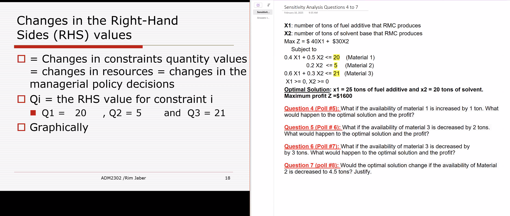
Page 18: Changes in RHS Values

• Impact of Changes in Constraints: Affect feasible region and optimal solution value

• RHS Values: e.g., Q1 = 20, Q2 = 5, Q3 = 21

Page 19: Optimal Solution Assessment

• Optimal Points: Evaluating through graphical representation

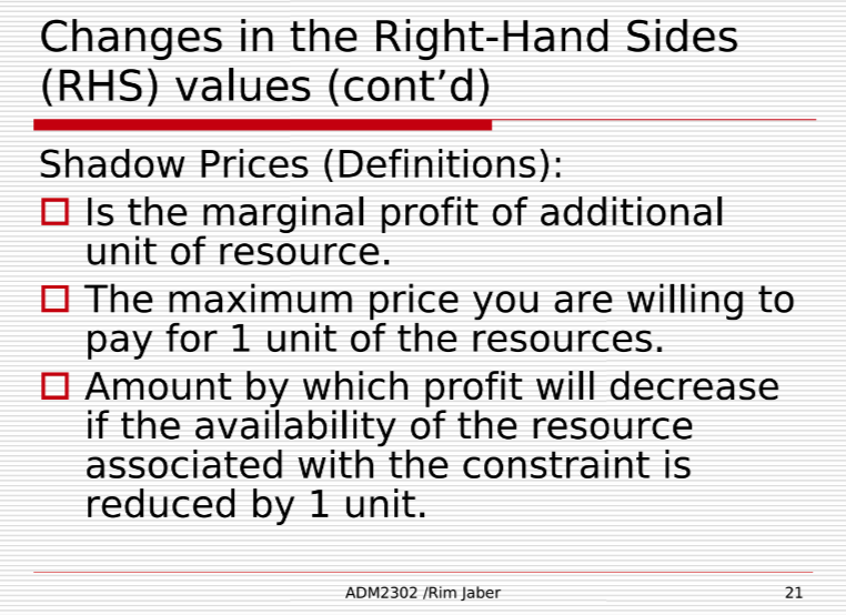
Page 20: Shadow Price Definition and Calculation

• Understanding Shadow Prices:

  • Increase profits per additional resource unit

• How to Determine: Increase RHS in spreadsheet, solve anew

Page 21: Shadow Prices in Context

• Definitions:

  • Marginal profit & max price willing for resources

  • Profit decreases by 1 unit reduction

Page 22: Purpose of RHS Value Analysis

• Objective: Examine small changes in RHS and their impact

Page 23: Range of Feasibility with RHS

• Value Ranges:

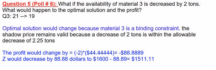
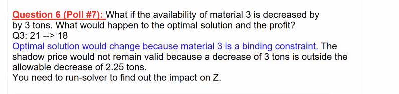
  • Q1: 14 ≤ Q1 ≤ 21.5

  • Q2: 4 ≤ Q2

  • Q3: 18.75 ≤ Q3 ≤ 30

Page 24: Changes Analysis of Binding vs Non-Binding Constraints

• Impact: Changes in binding constraints change optimal solution; non-binding do not affect profit unless within range

Page 25: Simultaneous Changes in Coefficients

• Purpose: Determine potential changes in optimal solution under multiple coefficient changes simultaneously

Page 26: 100 Percent Rule for Objective Function Coefficients

• Application: Total allowable changes must not exceed 100% to maintain optimal solution

Page 27: Example of 100 Percent Rule

• Illustration: c1 and c2 adjustments confirmed the stability of the current optimal solution

Page 28: Example of Exceeding 100 Percent Rule

• Outcome: Re-evaluate optimal solution needs resolving due to rule breach

Page 29: 100 Percent Rule for RHS

• Sum of changes: Assess RHS adjustments under feasibility ranges

Page 30: Class Discussion Summary

• Topic Validity and Examples discussed

Page 31: Reduced Cost Interpretation

• Concept: Explanation of reduced costs for unused activities; relevant for analysis and strategy

Page 32: Indicator of Multiple Optimal Solutions

• Criteria: Identifying zero optimal values and implications for solution stability

Page 33: Evaluating New Variables Introduction

• Sensitivity Report uses: Assessing the impact of variable changes on current production

Page 34: Proposing New Products for Production

• Example Evaluation of Ultra Base with material consumption and profit contribution

Page 35: Opportunity Cost Analysis

• Checking shadow price validity; guiding production decisions based on opportunity cost assessment

Page 36: Additional Discussions from Class

• Summary of solutions discussed in-depth during sessions

Page 37: Summary of Sensitivity Reports (Objective Function Coefficients)

• Final Values: Review usage and changes in objective coefficients

• Allowable Changes: Define operational ranges for coefficients

Page 38: Summary of Sensitivity Reports (Right-Hand-Sides)

• Final Values and Shadow Prices: Implications for resource adjustments and their operational impact.