
Eco101:Lecture8 -Perfectly Competitive Markets
Perfect Competition
1. Definition
A market structure characterized by multiple buyers and sellers.
Identical products mean individual seller actions do not influence the market price.
No constraints to firms entering or exiting the market exist.
Average Product of Labor= How much unit of labor is producing y/q divided by unit of labor
Marginal Product of Labor= Labor, increase the amount of labor by 1+, what is the effect on the additional unit? → Additional unit of output from hiring an additional unit of labor.
Average cost of production an additional unit of output? = Total Cost (Labor is the only input, and wage rate) . TC/ Labor= Average cost
Marginal Cost= Increase in total cost/Increase in outputMC = ΔTC/ΔQ
Relationship between MC and MP = inversely related. If Marginal Product (MP) rises, Marginal Cost (MC) falls, and vice versa
2. Key Features
?What makes a perfectly competitive market?
Mannnnny buyers + sellers of an IDENTICAL product (remember: actions do not influence market prices)
Price Takers: Each firm encounters a perfectly elastic demand curve at the market price.
Clarification: A perfectly elastic demand curve indicates that the quantity demanded by consumers will change infinitely with any change in price, meaning that firms in a perfectly competitive market can sell as much as they want at the market price but cannot influence the price with their own output levels.
Fixed number of firms in the short run; this number can change in the long run.
Insights
1) No barriers to entry → industry and firms are earning economic profit. If there is no barriers, these economic profits cannot persist. Positive profits → new firms entering the industry. Supply increases, price declines.
2)Any firm that is PC will take the price of given and there will be no influence on the market price ☹
Organic farmers
Setting:
You are an organic farmer (no pesticides) there is a sharp increase in the demand for organic foods
Questions:1. Will you earn (economic) profits? → Demand increases. Receive a higher price
Question:2. Will these (economic) profits persist over the long run? → no barriers to entry, supply curve will shift out , increase in quantity , reduction in price. Economic profits ❌❌🚫❌❌
Insight:For economic profits to persist over the long run, there must be obstacles
Question: A perfectly competitive firm, due to an increase in its costs, raises its price. As a result, the firm’s revenues:
3. Demand Curves
Market Demand (DD): The aggregate demand present in the market.
Individual Demand (dd): The demand for a specific firm, perfectly elastic.
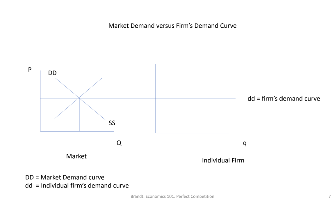
The line going through and down is the Equilibrium quantity and price
PE- Price equilibrium
QE- Quantity equilibrium.
4. Profit-Making Conditions
4.1 MR = P for Perfectly Competitive Firm
Marginal Revenue (MR) is equal to price (P).
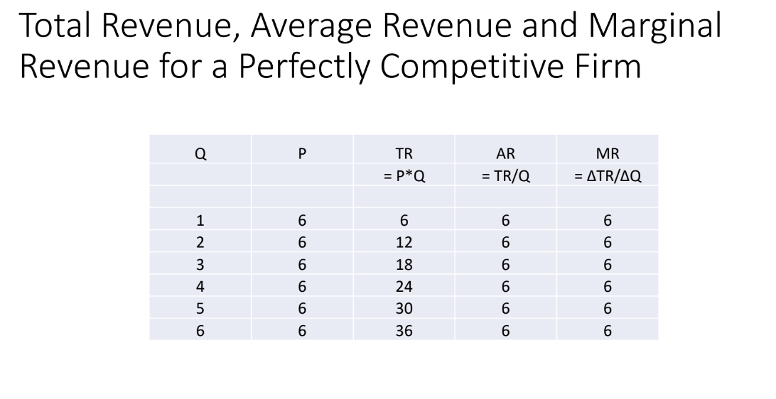
Total Revenue= At any level of output, 1 unit of output for $6 dollars. 6 × 1 , 6 × 2 , 6 × 3= 18 , 6 × 4 = 24 . . .
Average Revenue= Total Revenue divided by Quantity. 6/1, 12/2 = 6,
Marginal Revenue= The change in total revenue divided by the change in quantity.
Mathematical Example:Assuming a company sells widgets at a price of $6 each, let's calculate MR when the quantity sold increases from 3 to 4 units.
Calculate Total Revenue (TR) for each quantity sold:
At 3 units:TR = Price × QuantityTR = 6 × 3 = $18
At 4 units:TR = 6 × 4 = $24
Calculate the change in Total Revenue ( 24 - 18 = 6 ]
Calculate the change in Quantity Q = 4 - 3 = 1 ]
Now, substitute these values into the MR formula:[ MR = {6}{1} = 6 ]
For a Perfectly Competitive firm: MR= P
4.2 Profit Maximization
Firms produce where marginal cost (MC) meets marginal revenue (MR).
If P is greater than Average Variable Cost (AVC), the MC curve acts as the supply curve of the firm.
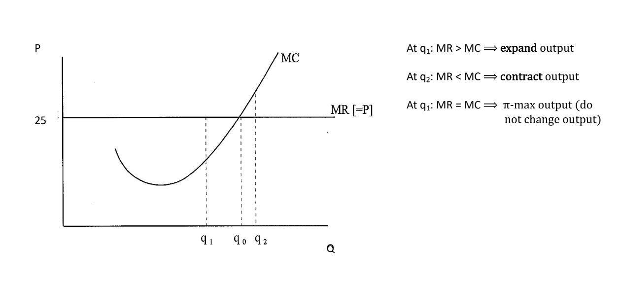
?What should the firm be comparing, to produce more? - Benefits [q1] , MR is greater than MC. If firm increases by one more unit/ output → able to increase their profits.
Suppose firm is producing [q2]→ MC of producing an additional unit is greater than the benefits. Is firm reduced their output then firm, you are able to increase your profits.
In both cases, your at a level where you can increase your profits.
MR=MC, profit-maximizing rule
MR=P, for perfectly-competitive firm
If the price is____ [, firm will supply___
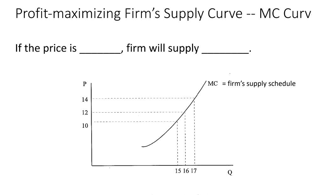
If Price is 10, then supply is 15
If price is 12, then supply is 16
If price is 14, supply is 17
5. Economic Profits and ATC
Economic profits are determined by Average Total Cost (ATC).Sustained economic profits attract firms into the market, eroding profits over time.
6. Entry and Exit
6.1 Short-run vs Long-run Equilibrium
In short-run equilibrium, firms may realize economic profits or losses.
In long-run equilibrium, firms achieve zero economic profit due to the dynamic entry and exit of firms.
6.2 Demand Shifts Impact
Demand fluctuations cause temporary profit changes that will stabilize over time.
7. Revenue Analysis
7.1 Total Revenue (TR), Average Revenue (AR), and Marginal Revenue (MR)
For a perfect competitor:
TR = P * Q
AR = TR / Q
MR = ΔTR / ΔQ
7.2 Elasticity of Demand Curve
The demand curve for a firm in a perfectly competitive market is perfectly elastic at the prevailing market price.
8. Profit Maximization Strategy
8.1 Output Decision
Increase output if MR exceeds MC.
Decrease output if MR is less than MC.Maintain output when MR equals MC.
9. Shutdown Point
Determined by comparing TR with Total Variable Costs (TVC).
If TR is less than TVC= shut down your company bbg to minimize ur loses
Firms will cease operations if TR is less than TVC; they must continue if TR exceeds TVC, even at a loss.
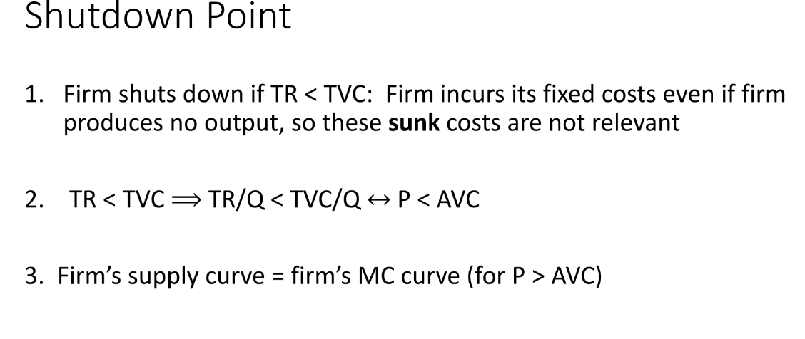
2) Total Revenue Divided by Quantity < Total Variable Cost/ Quantity is the same as P being less than Average Variable Cost
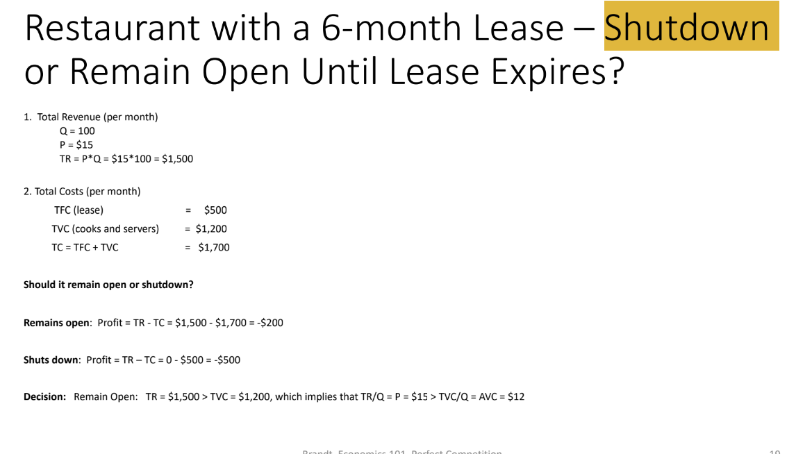
Restaurant with a 6-month Lease- Shutdown or Remain Open Until Lease Expires?
10. Long-run vs Short-run Comparisons
Firms can exits
New firms can enter
Short run→ Long run, Economic profits of the firm are key for these decisions.
Decisions to exit the market are based on long-term profit expectations; firms will enter if opportunities are present.
Zero economic profit indicates a normal profit situation with no motivation for market entry or exit.
Level of Profits
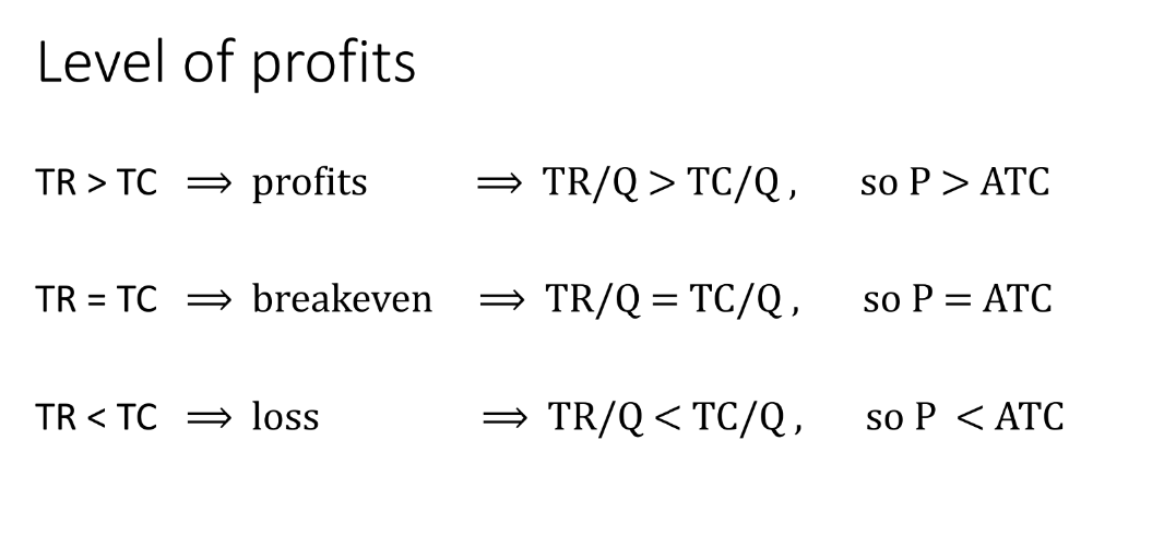
1) Economic profit (P>ATC)
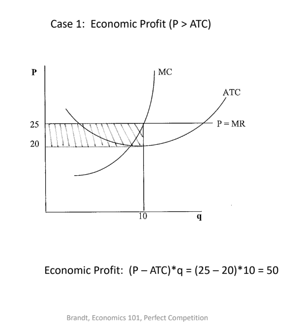
Is firm making money? Yes, the price is greater than the average total cost. the rectangle with the lines represent it?
2) Zero Economic Profit (P=ATC)
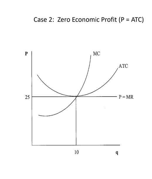
Firm is making not making any money
ATC= 25
Price =25
3) Economic Profit (P < ATC)
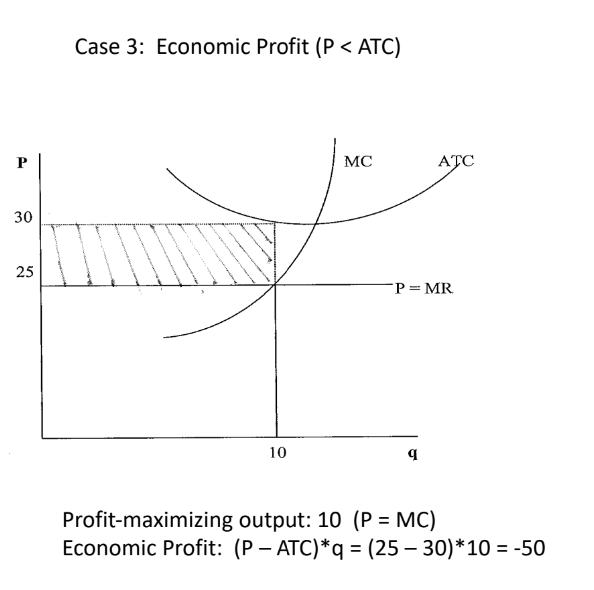
Firm is producing 10 units and is selling for 25
the Average total cost is equal to 30 which is less than the price.
Summary
11.1 Fluctuations in Market Price
If the price increases while firms are experiencing economic profits, this encourages new entries, which lowers market prices.
11.2 Industry Supply Responses
The supply curve shifts to the right as more firms enter due to the profits, ultimately leading to price reductions.
12. Long-run Industry Supply Curve
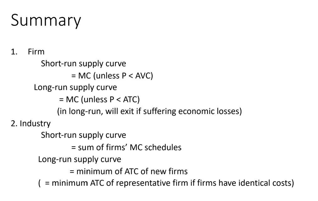
Demonstrates how ATC varies with the number of firms in constant cost industry scenarios.
Economic profits are driven to zero from entry and exit, what is the relationship between price and quantity supplied?
Case 1- All firms have identical cost schedules → Industry will be able to expand, new firms enter
Case 2-New entrants have higher costs → new firms will have higher costs , Long-run industry will rise,
Long-Run Equilibrium criteria
All firms is maximizing profits, Marginal Revenue = Marginal Cost
Zero economic profit because P=ATC
No incentive for firms to enter/ exit the industry.
Summary
13. Case Studies
13.1 Economic Profit Scenario
Profit can be defined as (P - ATC) multiplied by quantity (q) when P exceeds ATC.
13.2 Zero Economic Profit Scenario
If P equals ATC, firms secure normal profits with no incentives for entry or exit from the market.
13.3 Economic Loss Scenario
Losses occur when P is below ATC, prompting firms to consider market exit.
14. Summary of Decisions for Perfectly Competitive Firms
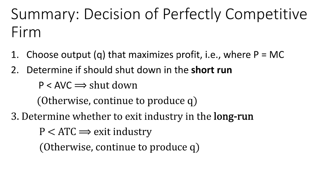
To maximize profits, produce at the output level where P equals MC.Evaluate TR against AVC for short-run shutdown decisions.Assess profitability against ATC for potential market exit in the long run.
15. Hot Dog Vendors Example
An increase in economic profits leads to market entry, shifting the supply curve to the right and reducing the market price.
Eco101:Lecture8 -Perfectly Competitive Markets
Perfect Competition
1. Definition
A market structure characterized by multiple buyers and sellers.
Identical products mean individual seller actions do not influence the market price.
No constraints to firms entering or exiting the market exist.
Average Product of Labor= How much unit of labor is producing y/q divided by unit of labor
Marginal Product of Labor= Labor, increase the amount of labor by 1+, what is the effect on the additional unit? → Additional unit of output from hiring an additional unit of labor.
Average cost of production an additional unit of output? = Total Cost (Labor is the only input, and wage rate) . TC/ Labor= Average cost
Marginal Cost= Increase in total cost/Increase in outputMC = ΔTC/ΔQ
Relationship between MC and MP = inversely related. If Marginal Product (MP) rises, Marginal Cost (MC) falls, and vice versa
2. Key Features
?What makes a perfectly competitive market?
Mannnnny buyers + sellers of an IDENTICAL product (remember: actions do not influence market prices)
Price Takers: Each firm encounters a perfectly elastic demand curve at the market price.
Clarification: A perfectly elastic demand curve indicates that the quantity demanded by consumers will change infinitely with any change in price, meaning that firms in a perfectly competitive market can sell as much as they want at the market price but cannot influence the price with their own output levels.
Fixed number of firms in the short run; this number can change in the long run.
Insights
1) No barriers to entry → industry and firms are earning economic profit. If there is no barriers, these economic profits cannot persist. Positive profits → new firms entering the industry. Supply increases, price declines.
2)Any firm that is PC will take the price of given and there will be no influence on the market price ☹
Organic farmers
Setting:
You are an organic farmer (no pesticides) there is a sharp increase in the demand for organic foods
Questions:1. Will you earn (economic) profits? → Demand increases. Receive a higher price
Question:2. Will these (economic) profits persist over the long run? → no barriers to entry, supply curve will shift out , increase in quantity , reduction in price. Economic profits ❌❌🚫❌❌
Insight:For economic profits to persist over the long run, there must be obstacles
Question: A perfectly competitive firm, due to an increase in its costs, raises its price. As a result, the firm’s revenues:
3. Demand Curves
Market Demand (DD): The aggregate demand present in the market.
Individual Demand (dd): The demand for a specific firm, perfectly elastic.

The line going through and down is the Equilibrium quantity and price
PE- Price equilibrium
QE- Quantity equilibrium.
4. Profit-Making Conditions
4.1 MR = P for Perfectly Competitive Firm
Marginal Revenue (MR) is equal to price (P).

Total Revenue= At any level of output, 1 unit of output for $6 dollars. 6 × 1 , 6 × 2 , 6 × 3= 18 , 6 × 4 = 24 . . .
Average Revenue= Total Revenue divided by Quantity. 6/1, 12/2 = 6,
Marginal Revenue= The change in total revenue divided by the change in quantity.
Mathematical Example:Assuming a company sells widgets at a price of $6 each, let's calculate MR when the quantity sold increases from 3 to 4 units.
Calculate Total Revenue (TR) for each quantity sold:
At 3 units:TR = Price × QuantityTR = 6 × 3 = $18
At 4 units:TR = 6 × 4 = $24
Calculate the change in Total Revenue ( 24 - 18 = 6 ]
Calculate the change in Quantity Q = 4 - 3 = 1 ]
Now, substitute these values into the MR formula:[ MR = {6}{1} = 6 ]
For a Perfectly Competitive firm: MR= P
4.2 Profit Maximization
Firms produce where marginal cost (MC) meets marginal revenue (MR).
If P is greater than Average Variable Cost (AVC), the MC curve acts as the supply curve of the firm.

?What should the firm be comparing, to produce more? - Benefits [q1] , MR is greater than MC. If firm increases by one more unit/ output → able to increase their profits.
Suppose firm is producing [q2]→ MC of producing an additional unit is greater than the benefits. Is firm reduced their output then firm, you are able to increase your profits.
In both cases, your at a level where you can increase your profits.
MR=MC, profit-maximizing rule
MR=P, for perfectly-competitive firm
If the price is____ [, firm will supply___

If Price is 10, then supply is 15
If price is 12, then supply is 16
If price is 14, supply is 17
5. Economic Profits and ATC
Economic profits are determined by Average Total Cost (ATC).Sustained economic profits attract firms into the market, eroding profits over time.
6. Entry and Exit
6.1 Short-run vs Long-run Equilibrium
In short-run equilibrium, firms may realize economic profits or losses.
In long-run equilibrium, firms achieve zero economic profit due to the dynamic entry and exit of firms.
6.2 Demand Shifts Impact
Demand fluctuations cause temporary profit changes that will stabilize over time.
7. Revenue Analysis
7.1 Total Revenue (TR), Average Revenue (AR), and Marginal Revenue (MR)
For a perfect competitor:
TR = P * Q
AR = TR / Q
MR = ΔTR / ΔQ
7.2 Elasticity of Demand Curve
The demand curve for a firm in a perfectly competitive market is perfectly elastic at the prevailing market price.
8. Profit Maximization Strategy
8.1 Output Decision
Increase output if MR exceeds MC.
Decrease output if MR is less than MC.Maintain output when MR equals MC.
9. Shutdown Point
Determined by comparing TR with Total Variable Costs (TVC).
If TR is less than TVC= shut down your company bbg to minimize ur loses
Firms will cease operations if TR is less than TVC; they must continue if TR exceeds TVC, even at a loss.

2) Total Revenue Divided by Quantity < Total Variable Cost/ Quantity is the same as P being less than Average Variable Cost
Restaurant with a 6-month Lease- Shutdown or Remain Open Until Lease Expires?

10. Long-run vs Short-run Comparisons
Firms can exits
New firms can enter
Short run→ Long run, Economic profits of the firm are key for these decisions.
Decisions to exit the market are based on long-term profit expectations; firms will enter if opportunities are present.
Zero economic profit indicates a normal profit situation with no motivation for market entry or exit.
Level of Profits

1) Economic profit (P>ATC)

Is firm making money? Yes, the price is greater than the average total cost. the rectangle with the lines represent it?
2) Zero Economic Profit (P=ATC)

Firm is making not making any money
ATC= 25
Price =25
3) Economic Profit (P < ATC)

Firm is producing 10 units and is selling for 25
the Average total cost is equal to 30 which is less than the price.
Summary

11.1 Fluctuations in Market Price
If the price increases while firms are experiencing economic profits, this encourages new entries, which lowers market prices.
11.2 Industry Supply Responses
The supply curve shifts to the right as more firms enter due to the profits, ultimately leading to price reductions.
12. Long-run Industry Supply Curve
Demonstrates how ATC varies with the number of firms in constant cost industry scenarios.
Economic profits are driven to zero from entry and exit, what is the relationship between price and quantity supplied?
Case 1- All firms have identical cost schedules → Industry will be able to expand, new firms enter
Case 2-New entrants have higher costs → new firms will have higher costs , Long-run industry will rise,
Long-Run Equilibrium criteria
All firms is maximizing profits, Marginal Revenue = Marginal Cost
Zero economic profit because P=ATC
No incentive for firms to enter/ exit the industry.
Summary

13. Case Studies
13.1 Economic Profit Scenario
Profit can be defined as (P - ATC) multiplied by quantity (q) when P exceeds ATC.
13.2 Zero Economic Profit Scenario
If P equals ATC, firms secure normal profits with no incentives for entry or exit from the market.
13.3 Economic Loss Scenario
Losses occur when P is below ATC, prompting firms to consider market exit.
14. Summary of Decisions for Perfectly Competitive Firms
To maximize profits, produce at the output level where P equals MC.Evaluate TR against AVC for short-run shutdown decisions.Assess profitability against ATC for potential market exit in the long run.
15. Hot Dog Vendors Example
An increase in economic profits leads to market entry, shifting the supply curve to the right and reducing the market price.