Advanced Applied Statistics
Bayes Theorem
Prior =
Likelihood =
Jeffreys Prior
The Fisher information is
The Jeffreys’ uninformative prior is given by:
Jeffreys prior is used whenever there is not a good reason to use another prior
Conjugate priors
Connection to exponential families
For certain likelihood functions, selecting a specific prior results in the posterior sharing the same distribution as the prior. This type of prior is then called a conjugate prior because it is conjugate to the likelihood.
Empirical Bayes
Know the standard approach
Baseball example
The uncertainty of low counts ½ is not the same as 50/100 since there is much more uncertainty in the first ½ than the second
1. step: Estimate a prior for the data by fitting the data to a chosen distribution by for example using maximum likelihood estimation (In this example using a Beta distribution)
2. step: Use that distribution as a prior for each individual estimate
This is a shrinkage method where uncertain observations move a lot towards the average and certain observations do not move that much.
Robbins Formula
With no knowledge about the prior density it is possible to estimate it using data
Objective Bayes
BIC - Bayes Information Criterion
A criterion for model selection
Introduces a penalty term for the number of parameters in the model
models with lower BIC values are preferred over models with higher BIC values
Alternative is AIC Akaike information criterion wich drops the penalty on the number of parameters / sample size
MCMC - Markov Chain Monte Carlo
Start with a current state theta_current
Propose a new state theta_new based on a proposal distribution
Calculate the acceptance probability which is a function of the likelihoods of the new and current states and the proposal distribution
Generate a random number u from a uniform distribution over [0, 1].
if accept the new state else retain current state
Repeat the steps for a large number of iterations to generate a chain of samples.
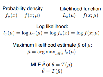
Maximum likelihood estimation
Maximum likelihood estimation
Steps in the maximum likelihood estimation:
Choose a likelihood function. A distribution that the parameters should be estimated
Take the log of the PDF of the likelihood function
Differentiate the logarithm of the likelihood function with respect to the model parameters: This gives the score function, which is a vector of partial derivatives of the logarithm of the likelihood function with respect to each model parameter
Set the score function equal to zero and solve for the model parameters: This gives the maximum likelihood estimates of the model parameters
Score function
The score function is the derivative of the log-likelihood function
The score function indicates how much the log-likelihood changes if you vary the
parameter estimate by an infinitesimal amount, given data x
The variance of the score is called the Fisher information
Fisher Information
It is defined as the variance of the score function, or the expected value of the observed information
The observed information is a sample-based version of the Fisher information, and it is used to estimate the Fisher information 3. The Fisher information is a theoretical measure of the amount of information that an observable random variable carries about an unknown parameter of a distribution that models the variable
Expectation of score:
Higher Fisher information is good
Observed Fisher information
It is the negative of the second derivative of the log-likelihood function with respect to the model parameters
Cramér Rao lower bound
Cramér-Rao: Any unbiased estimator θ-hat must have variance at least equal to the reciprocal of the Fisher information:
Conditional inference
Experiments which were not actually performed are statistically irrelevant.
Ancillary statistics: A statistic that contains “no direct information by itself”, but describes the experiment that was performed. Eg sample size
In conditional inference, we condition on the ancillary statistics, hoping to draw inferences that are simpler and more relevant.
Randomisation
Exponential families
From video
From book
a non negative volume of x which might make some x-values more likely regardless of theta. Will often just be 1 | |
Sufficient statistics. Vector measuring everything within x that matter for determining the probability for the parameters | |
The normalizer → ensure that the probability sum to 1 if you integrate over the domain of x | |
The parameter vector |
Parametric families
Basic univariate families
Normal
Poison
Binomial
Gamma
Beta
Multivariate normal distribution
is a gaussian in p dimensions
Σ is a real symmetric positive definite matrix, called the covariance matrix.
Because of Gaussian integral identities, you con obtain the following analytically:
The conditional distribution of a Gaussian is also Gaussian.
The marginal distribution of a Gaussian is also Gaussian
Law of large numbers
The law of large numbers says that if we sample from a distribution with a finite expectation, then the sample means will converge in probability (at least) to the population mean.
Central Limit Theorem
The sample mean of a large random sample of random variables with mean µ and finite variance σ2 has approximately a normal distribution with mean µ and variance σ 2/n.
Generalised Linear models
Logistic regression
Predicting either 0 or 1
s shape from 0 to 1
Using MLE to find the curve that give the maximum likelihood
The underlying exponential family is the binomial distribution. Binomial distribution: Probability of k successes in n trials, given an independent success probability of π.
Poison regression
Also uses a maximum likelihood estimation to find the best fit, however in this case it is just using a poisson distribution
Used when data are counts and always non negative
Generalised linear models
GLMs are a principled way to apply regression to quantities that are not normally distributed. Data are from a one-parameter exponential family
Fitting linear data
In the general case X is a vector
Deviance
The deviance between two densities f1(x) and f2(x) is a measure of how different the two distributions are.
Expectation Maximization
Gaussian Mixture Models
Assumes that data points come from k Gaussians with unknown parameters
Expectation and maximization models
The Expectation-Maximization (EM) algorithm is an iterative method used to estimate the parameters of a GMM
E and M step:
E step:
“completes the data” by assigning (expected) values to hidden variables.
M step:
Updates the model by maximising the expected log-likelihood
Latent variables:
Latent (or hidden) variables are random variables that facilitate the description of the model, but that you don’t have access to.
Survival Analysis
Life tables & Hazard rates
X is the year of death
fi = P(X = i) is the probability of dying at age i.
is the probability of surviving past age i.
The hazard rate at age i is the probability of dying at age i given you made it to age i − 1.
Survival age past j given survival past i − 1:
The Kaplan Meier Estimate
The Kaplan-Meier estimator is a non-parametric statistic used to estimate the survival function from lifetime data.
Let t(1) < t(2) < ... < t(n) be the ordered survival times. The Kaplan Meier formula estimates the survival probability as
where t is a time when at least one event happened, k is the number of events (e.g., deaths) that happened at time ti, and ni is the individuals known to have survived
The log-rank test
The Log-Rank test is good at getting a quantitative estimate of how likely it is that one treatment is better than another.
Statistical hypothesis test used to compare the survival distributions of two or more groups.
It is a non-parametric test
Non-parametric methods
a type of statistical analysis that makes minimal assumptions about the underlying distribution of the data being studied
Parametric Bootstrap
Assumes the data follows a specific distribution
Samples the same way as the non-parametric bootstrap
Choose a parametric model
Estimate parameters based on the given sample set.
Generate new samples of the model
Calculate the statistic.
Non-parametric Bootstrap
Does not assume that data comes from a specific distribution
Sampling with replacement
Original data should be a reasonable representation of the population
Bootstrap and calculate some relevant statistic on each sample
Bootstrap confidence intervals
Bootstrap samples
Calculate relevant statistic on the sample, R^2 from a regression or median or mean
The percentile method: Calculate the 95% confidence interval of the relevant statistic fx by taking the 2.5 and 97.5 percentiles
Bootstrap error:
The standard deviation of the mean/median calculated from the bootstrap
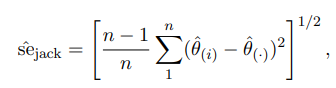
Jackknife-Estimate
When the underlying distribution is unknown
Leave one out resampling
Removing the i’th sample for i in length observations
The standard error is n-1 because we remove 1 obs in all samples.
Neymans construction
Repeated Sampling: Draw multiple samples and compute a confidence interval from each sample.
Visualize Intervals: Plot all intervals—those covering the true parameter are one color (e.g., green), those missing it are another (e.g., red).
Frequentist Interpretation: In the long run, the proportion of intervals containing the true parameter matches the confidence level (e.g., 95% of intervals contain the true value for a 95% confidence interval).
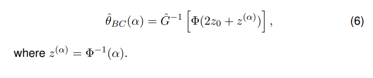
Bias adjusted confidence interval
Calculate the bias-correction parameter, z0, by finding the value of the standard normal distribution that corresponds to the percentile of the bootstrap distribution that contains the original estimate.
where Φ is the cdf of the normal distribution
Calculate the acceleration parameter, a, by finding the value of the standard normal distribution that corresponds to the percentile of the bootstrap distribution that contains the z0 value.
The bias corrected (BC) confidence interval endpoint is defined as:
Bootstrap-t intervals
Take n many bootstrap samples from the original dataset.
For each sample, calculate the mean.
Calculate the standard error of the distribution of means from the bootstrap samples.
Calculate the t-value for the desired level of confidence and degrees of freedom.
Multiply the standard error by the t-value and add and subtract the resulting value from the sample mean to obtain the confidence interval.
Confidence intervals
Suppose you know the underlying process, given by fµ(x). The 95% confidence interval is obtained by finding the values of xmin and xmax such that P(X > x) ≤ .025 and/or P(X < x) ≤ .025.
Example: the normal distribution with µ = 0 and σ = 1:
P(X < x) = 0.025 → x ≈ −1.96
P(X > x) = 0.025 → x ≈ 1.96
Cross-validation
Prediction problems
A normal ML prediction problem
The input consists of a set of predictors (xi) and the output consists of a set of responses (yi). The goal is to find a function rd(x) that accurately predicts the response y for a given new predictor x.
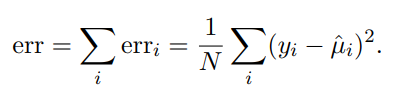
The overall prediction error (quantifying prediction error)
An error that maps whether the prediction was correct or not
Most common squared error with continuous numbers:
with y-hat being the prediction and y being the actual value
And in the discrete case the most used is:
Cross-validation in general
Non-parametric method
When a part of the training set is held out as the validation set
Err = EF {D(y0, yˆ0)} for a new case obtained independently of d.
If we can spare some samples from the training set, then we can define a validation set dval = {(x0i, y0i)} and define the unbiased estimate;
The cross-validation estimate of prediction error is;
Covariance penalties
The covariance penalty approach treats prediction error estimation in a regression framework.
It is based on the covariance between data points and their corresponding prediction
In the context of the covariance penalty, it is used to measure the relationship between the observed values of the dependent variable and the predicted values of the dependent variable
The overall prediction error is assessed in terms of the squared discrepancy:
where the expectation is given by;
The overall prediction error is estimated by as;
The linear model and Mallows Cp estimate
Is used to estimate the prediction error of a linear regression model.
applied in the context of model selection, where a number of predictor variables are available for predicting some outcome, and the goal is to find the best model involving a subset of these predictors. A small value of Cp means that the model is relatively precise.
This formula is called Mallows’ Cp estimate of prediction error. For least squared estimation, M = X(XT X) −1XT has tr[M] = p, the number of predictors, so;
Hypothesis testing
Null hypothesis - Rejected if p< alpha level set
alternative hypothesis - The hypothesis accepted if H0 is rejected
Collect unbiased samples and make a statistical test on the data
Type 1 error false positive:
Null hypothesis was rejected, but shouldn’t have been
Type 2 error:
Null hypothesis should have been rejected, but wasn’t.
Different tests:
Z-test: A z-test is used to test the mean of a population when the population standard deviation is known
T-test: A t-test is used to test the mean of a population when the population standard deviation is unknown
Chi-squared test: A chi-squared test is used to test the independence of two categorical variables
Mann-Whitney U test: The Mann-Whitney U test is another nonparametric test used to compare two independent samples
Kolmogorov-Smirnov test: The Kolmogorov-Smirnov test is used to test whether two samples come from the same distribution
Fisher’s exact test: Fisher’s exact test is used to test the independence of two categorical variables when the sample size is small
Large scale testing
When testing many hypotheses
Will give many false positive (type 1 errors)
If we ignore them, we’ll make many Type II errors (lose power).
How to balance between type 1 and type 2 errors when testing multiple hypotheses?
Bonferroni correction
Divide significance level α by number of tests N, test each hypothesis at level α/N.
Very conservative for large N
Holm’s procedure
Uniformly more powerful than Bonferroni bound.
The procedure:
Order observed p-values from smallest to largest
For each p-value:
reject the i’th null hypothesis if the p value < α/(N − i + 1)
family-wise error rate
FWER - Probability of making a type 1 error among a specified group or “family” of tests.
False-discovery rate
Poportion of false posivites among all significant results
The false-discovery rate (FDR) of a decision procedure D is its expected false-discovery proportion.
Controlling the FDR increases the power of our tests while still keeping Type I error under (less stringent) control.
FDR control is less conservative than FWER control.
Fdp: false-discovery proportion
Is unobservable
Benjamini-Hochberg procedure
Used to control the FDR
Arrange the p-values in order from smallest to largest, assigning a rank to each one – the smallest p-value has a rank of 1, the next smallest has a rank of 2, etc.
q= the chosen false discovery rate.
Find the largest p-value that is less than the critical value. Designate every p-value that is smaller than this p-value to be significant.
Two group model
The two-groups model is a simple Bayesian construction that is used to estimate the distribution of the null hypothesis. It is used to calculate the probability of observing a certain number of false positives, given the number of tests performed
f(z) = π0f0(z) + π1f1(z)
π0: Prior probability of null hypothesis being true.
π1 = 1 − π0: Prior probability of alternative being true.
Test statistics where H0 is true are drawn iid from density f0(z) with cdf F0(z).
Test statistics where H1 is true are drawn iid from density f1(z) with cdf F1(z).
Local fdr
local false-discovery rate
Is a Bayesian approach that provides a more refined measure of significance than the traditional false discovery rate (FDR)
The lfdrs defined as the probability that a null hypothesis is true, given that it has been rejected by a statistical test.
null distribution
The main point of using the empirical null distribution is to estimate the distribution of the null hypothesis.
Is used to calculate the probability of observing a certain number of false positives (type 1 error), given the number of tests performed
null estimation
James Stein Estimator
Shrinkage estimation
Shrinkage estimation is a statistical technique that involves “shrinking” extreme values in a sample towards a central value, such as the sample mean, to obtain a better estimate of the true population mean
James-Stein Estimator
The James-Stein estimator is a statistical technique that involves “shrinking” extreme values in a sample towards a central value, such as the sample mean, to obtain a better estimate of the true population mean
Least squares estimator
When using least squares to find the best fitting line
X is the design matrix, and y is the response vector
The design matrix is a matrix of values of explanatory variables of a set of objects. Each row represents an individual object, with the successive columns corresponding to the variables and their specific values for that object.
Ridge Regression
Ridge Regression
Ridge regression is linear regression with squared loss and a penalty on the `2-norm of β
Effects of ridge regression:
Biased parameter estimates: Estimated coefficients are shrunk towards zero.
The model requires “stronger evidence” to grow the weights.
Avoids overfitting.
Potentially better performance on new datasets.
Ridge regression overcomes the problem of overfitting by adding a shrinkage penalty term to the least squares objective function, which shrinks the magnitude of the regression coefficients towards zero. This results in a more stable and generalizable model that is less prone to overfitting.
Standardization in Ridge Regression
In Ridge Regression it is important to standardize all variables
Otherwise some higher variables might be overly influential
Sparse Modeling and the Lasso
Best subset regression
Best subset regression is a variable selection method that involves fitting all possible regression models derived from all possible combinations of the candidate predictors, and then selecting the subset of predictors that do the best at meeting some well-defined objective criterion, such as having the largest R^2-value or the smallest MSE
Forward stepwise regression
Forward stepwise regression is a variable selection method that starts with a model that contains no variables (called the Null Model) and then adds the most significant variables one after the other until a pre-specified stopping rule is reached or until all the variables under consideration are included in the model.
The most significant value can be determined by different measures for example by when adding to the model;
It has the smallest p-value, or
It provides the highest increase in R^2
The stopping rule is satisfied when all remaining variables to consider have a p-value larger than some specified threshold, if added to the model.
Lasso regression
LASSO regression uses squared loss and a penalty on the l1 norm of β.
Regularization
We want our models to learn generalisable patterns, not idiosyncrasies of samples.
Key idea of regularization: Limit the capacity of the model, so it only learns patterns for which it has good evidence.
L1 and L2 norms
L1 norm:
Also Lasso regression
L2 norm:
Also Ridge regression
What is the difference between Bayesian and Frequentist approach?
What is the difference between parametric and non-parametric methods?
Bayes Theorem
Prior =
Likelihood =
Jeffreys Prior
The Fisher information is
The Jeffreys’ uninformative prior is given by:
Jeffreys prior is used whenever there is not a good reason to use another prior
Conjugate priors
Connection to exponential families
For certain likelihood functions, selecting a specific prior results in the posterior sharing the same distribution as the prior. This type of prior is then called a conjugate prior because it is conjugate to the likelihood.
Empirical Bayes
Know the standard approach
Baseball example
The uncertainty of low counts ½ is not the same as 50/100 since there is much more uncertainty in the first ½ than the second
1. step: Estimate a prior for the data by fitting the data to a chosen distribution by for example using maximum likelihood estimation (In this example using a Beta distribution)
2. step: Use that distribution as a prior for each individual estimate
This is a shrinkage method where uncertain observations move a lot towards the average and certain observations do not move that much.
Robbins Formula
With no knowledge about the prior density it is possible to estimate it using data
Objective Bayes
BIC - Bayes Information Criterion
A criterion for model selection
Introduces a penalty term for the number of parameters in the model
models with lower BIC values are preferred over models with higher BIC values
Alternative is AIC Akaike information criterion wich drops the penalty on the number of parameters / sample size
MCMC - Markov Chain Monte Carlo
Start with a current state theta_current
Propose a new state theta_new based on a proposal distribution
Calculate the acceptance probability which is a function of the likelihoods of the new and current states and the proposal distribution
Generate a random number u from a uniform distribution over [0, 1].
if accept the new state else retain current state
Repeat the steps for a large number of iterations to generate a chain of samples.
Maximum likelihood estimation
Maximum likelihood estimation
Steps in the maximum likelihood estimation:
Choose a likelihood function. A distribution that the parameters should be estimated
Take the log of the PDF of the likelihood function
Differentiate the logarithm of the likelihood function with respect to the model parameters: This gives the score function, which is a vector of partial derivatives of the logarithm of the likelihood function with respect to each model parameter
Set the score function equal to zero and solve for the model parameters: This gives the maximum likelihood estimates of the model parameters
Score function
The score function is the derivative of the log-likelihood function
The score function indicates how much the log-likelihood changes if you vary the
parameter estimate by an infinitesimal amount, given data x
The variance of the score is called the Fisher information
Fisher Information
It is defined as the variance of the score function, or the expected value of the observed information
The observed information is a sample-based version of the Fisher information, and it is used to estimate the Fisher information 3. The Fisher information is a theoretical measure of the amount of information that an observable random variable carries about an unknown parameter of a distribution that models the variable
Expectation of score:
Higher Fisher information is good
Observed Fisher information
It is the negative of the second derivative of the log-likelihood function with respect to the model parameters
Cramér Rao lower bound
Cramér-Rao: Any unbiased estimator θ-hat must have variance at least equal to the reciprocal of the Fisher information:
Conditional inference
Experiments which were not actually performed are statistically irrelevant.
Ancillary statistics: A statistic that contains “no direct information by itself”, but describes the experiment that was performed. Eg sample size
In conditional inference, we condition on the ancillary statistics, hoping to draw inferences that are simpler and more relevant.
Randomisation
Exponential families
From video
From book
a non negative volume of x which might make some x-values more likely regardless of theta. Will often just be 1 | |
Sufficient statistics. Vector measuring everything within x that matter for determining the probability for the parameters | |
The normalizer → ensure that the probability sum to 1 if you integrate over the domain of x | |
The parameter vector |
Parametric families
Basic univariate families
Normal
Poison
Binomial
Gamma
Beta
Multivariate normal distribution
is a gaussian in p dimensions
Σ is a real symmetric positive definite matrix, called the covariance matrix.
Because of Gaussian integral identities, you con obtain the following analytically:
The conditional distribution of a Gaussian is also Gaussian.
The marginal distribution of a Gaussian is also Gaussian
Law of large numbers
The law of large numbers says that if we sample from a distribution with a finite expectation, then the sample means will converge in probability (at least) to the population mean.
Central Limit Theorem
The sample mean of a large random sample of random variables with mean µ and finite variance σ2 has approximately a normal distribution with mean µ and variance σ 2/n.
Generalised Linear models
Logistic regression
Predicting either 0 or 1
s shape from 0 to 1
Using MLE to find the curve that give the maximum likelihood
The underlying exponential family is the binomial distribution. Binomial distribution: Probability of k successes in n trials, given an independent success probability of π.
Poison regression
Also uses a maximum likelihood estimation to find the best fit, however in this case it is just using a poisson distribution
Used when data are counts and always non negative
Generalised linear models
GLMs are a principled way to apply regression to quantities that are not normally distributed. Data are from a one-parameter exponential family
Fitting linear data
In the general case X is a vector
Deviance
The deviance between two densities f1(x) and f2(x) is a measure of how different the two distributions are.
Expectation Maximization
Gaussian Mixture Models
Assumes that data points come from k Gaussians with unknown parameters
Expectation and maximization models
The Expectation-Maximization (EM) algorithm is an iterative method used to estimate the parameters of a GMM
E and M step:
E step:
“completes the data” by assigning (expected) values to hidden variables.
M step:
Updates the model by maximising the expected log-likelihood
Latent variables:
Latent (or hidden) variables are random variables that facilitate the description of the model, but that you don’t have access to.
Survival Analysis
Life tables & Hazard rates
X is the year of death
fi = P(X = i) is the probability of dying at age i.
is the probability of surviving past age i.
The hazard rate at age i is the probability of dying at age i given you made it to age i − 1.
Survival age past j given survival past i − 1:
The Kaplan Meier Estimate
The Kaplan-Meier estimator is a non-parametric statistic used to estimate the survival function from lifetime data.
Let t(1) < t(2) < ... < t(n) be the ordered survival times. The Kaplan Meier formula estimates the survival probability as
where t is a time when at least one event happened, k is the number of events (e.g., deaths) that happened at time ti, and ni is the individuals known to have survived
The log-rank test
The Log-Rank test is good at getting a quantitative estimate of how likely it is that one treatment is better than another.
Statistical hypothesis test used to compare the survival distributions of two or more groups.
It is a non-parametric test
Non-parametric methods
a type of statistical analysis that makes minimal assumptions about the underlying distribution of the data being studied
Parametric Bootstrap
Assumes the data follows a specific distribution
Samples the same way as the non-parametric bootstrap
Choose a parametric model
Estimate parameters based on the given sample set.
Generate new samples of the model
Calculate the statistic.
Non-parametric Bootstrap
Does not assume that data comes from a specific distribution
Sampling with replacement
Original data should be a reasonable representation of the population
Bootstrap and calculate some relevant statistic on each sample
Bootstrap confidence intervals
Bootstrap samples
Calculate relevant statistic on the sample, R^2 from a regression or median or mean
The percentile method: Calculate the 95% confidence interval of the relevant statistic fx by taking the 2.5 and 97.5 percentiles
Bootstrap error:
The standard deviation of the mean/median calculated from the bootstrap
Jackknife-Estimate
When the underlying distribution is unknown
Leave one out resampling
Removing the i’th sample for i in length observations
The standard error is n-1 because we remove 1 obs in all samples.
Neymans construction
Repeated Sampling: Draw multiple samples and compute a confidence interval from each sample.
Visualize Intervals: Plot all intervals—those covering the true parameter are one color (e.g., green), those missing it are another (e.g., red).
Frequentist Interpretation: In the long run, the proportion of intervals containing the true parameter matches the confidence level (e.g., 95% of intervals contain the true value for a 95% confidence interval).
Bias adjusted confidence interval
Calculate the bias-correction parameter, z0, by finding the value of the standard normal distribution that corresponds to the percentile of the bootstrap distribution that contains the original estimate.
where Φ is the cdf of the normal distribution
Calculate the acceleration parameter, a, by finding the value of the standard normal distribution that corresponds to the percentile of the bootstrap distribution that contains the z0 value.
The bias corrected (BC) confidence interval endpoint is defined as:
Bootstrap-t intervals
Take n many bootstrap samples from the original dataset.
For each sample, calculate the mean.
Calculate the standard error of the distribution of means from the bootstrap samples.
Calculate the t-value for the desired level of confidence and degrees of freedom.
Multiply the standard error by the t-value and add and subtract the resulting value from the sample mean to obtain the confidence interval.
Confidence intervals
Suppose you know the underlying process, given by fµ(x). The 95% confidence interval is obtained by finding the values of xmin and xmax such that P(X > x) ≤ .025 and/or P(X < x) ≤ .025.
Example: the normal distribution with µ = 0 and σ = 1:
P(X < x) = 0.025 → x ≈ −1.96
P(X > x) = 0.025 → x ≈ 1.96
Cross-validation
Prediction problems
A normal ML prediction problem
The input consists of a set of predictors (xi) and the output consists of a set of responses (yi). The goal is to find a function rd(x) that accurately predicts the response y for a given new predictor x.
The overall prediction error (quantifying prediction error)
An error that maps whether the prediction was correct or not
Most common squared error with continuous numbers:
with y-hat being the prediction and y being the actual value
And in the discrete case the most used is:
Cross-validation in general
Non-parametric method
When a part of the training set is held out as the validation set
Err = EF {D(y0, yˆ0)} for a new case obtained independently of d.
If we can spare some samples from the training set, then we can define a validation set dval = {(x0i, y0i)} and define the unbiased estimate;
The cross-validation estimate of prediction error is;
Covariance penalties
The covariance penalty approach treats prediction error estimation in a regression framework.
It is based on the covariance between data points and their corresponding prediction
In the context of the covariance penalty, it is used to measure the relationship between the observed values of the dependent variable and the predicted values of the dependent variable
The overall prediction error is assessed in terms of the squared discrepancy:
where the expectation is given by;
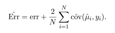
The overall prediction error is estimated by as;
The linear model and Mallows Cp estimate
Is used to estimate the prediction error of a linear regression model.
applied in the context of model selection, where a number of predictor variables are available for predicting some outcome, and the goal is to find the best model involving a subset of these predictors. A small value of Cp means that the model is relatively precise.
This formula is called Mallows’ Cp estimate of prediction error. For least squared estimation, M = X(XT X) −1XT has tr[M] = p, the number of predictors, so;
Hypothesis testing
Null hypothesis - Rejected if p< alpha level set
alternative hypothesis - The hypothesis accepted if H0 is rejected
Collect unbiased samples and make a statistical test on the data
Type 1 error false positive:
Null hypothesis was rejected, but shouldn’t have been
Type 2 error:
Null hypothesis should have been rejected, but wasn’t.
Different tests:
Z-test: A z-test is used to test the mean of a population when the population standard deviation is known
T-test: A t-test is used to test the mean of a population when the population standard deviation is unknown
Chi-squared test: A chi-squared test is used to test the independence of two categorical variables
Mann-Whitney U test: The Mann-Whitney U test is another nonparametric test used to compare two independent samples
Kolmogorov-Smirnov test: The Kolmogorov-Smirnov test is used to test whether two samples come from the same distribution
Fisher’s exact test: Fisher’s exact test is used to test the independence of two categorical variables when the sample size is small
Large scale testing
When testing many hypotheses
Will give many false positive (type 1 errors)
If we ignore them, we’ll make many Type II errors (lose power).
How to balance between type 1 and type 2 errors when testing multiple hypotheses?
Bonferroni correction
Divide significance level α by number of tests N, test each hypothesis at level α/N.
Very conservative for large N
Holm’s procedure
Uniformly more powerful than Bonferroni bound.
The procedure:
Order observed p-values from smallest to largest
For each p-value:
reject the i’th null hypothesis if the p value < α/(N − i + 1)
family-wise error rate
FWER - Probability of making a type 1 error among a specified group or “family” of tests.
False-discovery rate
Poportion of false posivites among all significant results
The false-discovery rate (FDR) of a decision procedure D is its expected false-discovery proportion.
Controlling the FDR increases the power of our tests while still keeping Type I error under (less stringent) control.
FDR control is less conservative than FWER control.
Fdp: false-discovery proportion
Is unobservable
Benjamini-Hochberg procedure
Used to control the FDR
Arrange the p-values in order from smallest to largest, assigning a rank to each one – the smallest p-value has a rank of 1, the next smallest has a rank of 2, etc.
q= the chosen false discovery rate.
Find the largest p-value that is less than the critical value. Designate every p-value that is smaller than this p-value to be significant.
Two group model
The two-groups model is a simple Bayesian construction that is used to estimate the distribution of the null hypothesis. It is used to calculate the probability of observing a certain number of false positives, given the number of tests performed
f(z) = π0f0(z) + π1f1(z)
π0: Prior probability of null hypothesis being true.
π1 = 1 − π0: Prior probability of alternative being true.
Test statistics where H0 is true are drawn iid from density f0(z) with cdf F0(z).
Test statistics where H1 is true are drawn iid from density f1(z) with cdf F1(z).
Local fdr
local false-discovery rate
Is a Bayesian approach that provides a more refined measure of significance than the traditional false discovery rate (FDR)
The lfdrs defined as the probability that a null hypothesis is true, given that it has been rejected by a statistical test.
null distribution
The main point of using the empirical null distribution is to estimate the distribution of the null hypothesis.
Is used to calculate the probability of observing a certain number of false positives (type 1 error), given the number of tests performed
null estimation
James Stein Estimator
Shrinkage estimation
Shrinkage estimation is a statistical technique that involves “shrinking” extreme values in a sample towards a central value, such as the sample mean, to obtain a better estimate of the true population mean
James-Stein Estimator
The James-Stein estimator is a statistical technique that involves “shrinking” extreme values in a sample towards a central value, such as the sample mean, to obtain a better estimate of the true population mean
Least squares estimator
When using least squares to find the best fitting line
X is the design matrix, and y is the response vector
The design matrix is a matrix of values of explanatory variables of a set of objects. Each row represents an individual object, with the successive columns corresponding to the variables and their specific values for that object.
Ridge Regression
Ridge Regression
Ridge regression is linear regression with squared loss and a penalty on the `2-norm of β
Effects of ridge regression:
Biased parameter estimates: Estimated coefficients are shrunk towards zero.
The model requires “stronger evidence” to grow the weights.
Avoids overfitting.
Potentially better performance on new datasets.
Ridge regression overcomes the problem of overfitting by adding a shrinkage penalty term to the least squares objective function, which shrinks the magnitude of the regression coefficients towards zero. This results in a more stable and generalizable model that is less prone to overfitting.
Standardization in Ridge Regression
In Ridge Regression it is important to standardize all variables
Otherwise some higher variables might be overly influential
Sparse Modeling and the Lasso
Best subset regression
Best subset regression is a variable selection method that involves fitting all possible regression models derived from all possible combinations of the candidate predictors, and then selecting the subset of predictors that do the best at meeting some well-defined objective criterion, such as having the largest R^2-value or the smallest MSE
Forward stepwise regression
Forward stepwise regression is a variable selection method that starts with a model that contains no variables (called the Null Model) and then adds the most significant variables one after the other until a pre-specified stopping rule is reached or until all the variables under consideration are included in the model.
The most significant value can be determined by different measures for example by when adding to the model;
It has the smallest p-value, or
It provides the highest increase in R^2
The stopping rule is satisfied when all remaining variables to consider have a p-value larger than some specified threshold, if added to the model.
Lasso regression
LASSO regression uses squared loss and a penalty on the l1 norm of β.
Regularization
We want our models to learn generalisable patterns, not idiosyncrasies of samples.
Key idea of regularization: Limit the capacity of the model, so it only learns patterns for which it has good evidence.
L1 and L2 norms
L1 norm:
Also Lasso regression
L2 norm:
Also Ridge regression
What is the difference between Bayesian and Frequentist approach?
What is the difference between parametric and non-parametric methods?