Physics AT1 flashcards

This booklet will help you study for the Working Scientifically and Depth Study Assessment task - remember ALWAYS check how these skills have been done in the MHS booklet as this is what we will base our marking on...

Physics Skills in Experimentation

Stage 6 Physics – Working Scientifically Activity book

Contents

Unit

1

2

3

4A

4B

5

6

7

8

9

Topic

Units for measurement Significant figures

Scientific notation and orders of magnitude Linear regression

Advanced linear regression Accuracy and error

Estimating uncertainty in measurements

Assessing reliability in experiments

Estimating uncertainty in results

Assessing validity in experiments

Solutions

References

THIS BOOKLET HAS BEEN MODIFIED TO MATCH THE MHS SKILLS AND DEPTH STUDY BOOKLET FOR 2022.

Produced in the First Year Physics Unit School of Physics

The University of New South Wales, Sydney CRICOS Provider Number 00098G

©2020 The University of New South Wales

Introduction

This activity book is intended for students of the Stage 6 Physics course in New South Wales. It draws upon resources published by the NSW Department of Education in their Working Scientifically support documents as well as those from the First Year Physics Unit at the University of New South Wales, Sydney.

In this activity book, definitions and procedures used in physics research and tertiary study are streamlined and adapted for students of physics at high school level. Some ideas and techniques have been simplified so that secondary school students can access skills for experimental work.

This activity book is in no way intended to be prescriptive; teachers should consider the learning requirements and outcomes for their students when using this activity book with their students.

M de la Pena, 2020

References to the NSW Physics Stage 6 Syllabus

PH11/12-4 Processing data and information

A student selects and processes appropriate qualitative and quantitative data and information using a range of appropriate media.

PH11/12-5 Analysing data and information

A student analyses and evaluates primary and secondary data and information

(NSW Education Standards Authority, 2017)

– Units for measurement

Units add important information to measurements because a numerical value means nothing on its own.

A unit has to be an agreed quantity of a thing to be measured, because when we say or write down a measurement, we are actually giving a number of multiples of that unit. For example, when I tell you that the length of something is 3 metres, I am telling you that its length is 3 × 1 metre, and this will only be accurate if you agree with me about what a single metre is.

The agreed system of units used in science is the International System of units (SI units). The base units are:

All other units are based on these seven base units.

Question 1

What base SI units are used for the following physical quantities?

Question 2

There are many other units used in physics, but they are actually derived from the base units.

For example, the units of speed are derived from the units for length and time (metres per second):

speed = distance = 1 m = 1 m/s = 1 m s^-1

time 1 s

What are the derived units for the following physical quantities? Relevant equations have been included to help you.

Question 3

Some quantities are so special that their derived unit is given a name. For example, you might know the named unit for force – the newton (N). However, the unit for force is actually derived from the SI base units. Since force is determined by the equation

F = ma

the unit for force derived from base units is

1 newton = 1 kg × 1 m s^-2 = 1 kg m s^-2

Find out the named units for the quantities below. You can use the internet or references to find out.

Question 4

Some quantities are so big or small in scale that the units used to measure them are too big or too small to make sense of their size. Sometimes, a prefix is added to the unit make the written or spoken value more manageable and easier to conceptualise.

For example, 3 thousand metres is more conveniently written and spoken as 3 kilometres. Below is a table of SI prefixes and their multipliers.

1. Rewrite the following values in more convenient units

2. Rewrite the following values in terms of their base-sized unit.

Question 5

The units for mass have an interesting history. The fundamental unit for mass in the nineteenth-century metric system was the gram – a thousand grams being a kilogram. However, when SI units were established in 1960, the kilogram was chosen as the base unit because it was on the same kind of size scale as the other units, like the metre. Other units, like the tonne, also exist in metric systems of units.

Write the names of the convenient mass units based around the gram and kilogram.

– Significant figures

Significant figures are important because they convey the accuracy and uncertainty in a value. The last significant figure in a number suggests that the value is accurate to within ±½ of that place. For example:

• 120 m (2 significant figures) implies a length with uncertainty of 120 ± 5 m

  • 123 m (3 significant figures) implies a length with uncertainty of 123 ± 0.5 m

Rules for significant figures – what counts as a significant figure?

• Non-zero digits are significant.

• Trailing zeroes in a whole number are generally not significant (these zeroes are used to keep the other figures in their correct value places).

‒ 75000 m – the 7 and 5 are significant. There are 2 significant figures.

‒ 75420 m – the 7, 5, 4 and 2 are significant. There are 4 significant figures. There is less uncertainty in this number.

• Leading zeroes are not significant (these zeroes are used to keep the other figures in their correct value places).

‒ 0.000832 kg – only 8, 3, and 2 are significant. There are 3 significant figures.

• The zeroes between non-zero digits are significant.

‒ 90.04 s – each figure is significant. There are 4 significant figures.

• The trailing zeroes in a decimal are significant.

‒ 8.30 L – each figure is significant. There are 3 significant figures.

‒ 3.200 J – each figure is significant. There are 4 significant figures.

The result of a calculation is only as accurate as the least accurate number used to compute it. When reporting the result of a calculation, the result must be rounded to the same number of figures as the smallest number of significant figures used in the calculation. For example

Energy = 3.457 W × 5.60 s = 19.3292 J

the answer can only be reported as 19.3 J because the smallest number of significant figures in the calculation was three.

Question 1

How many significant figures are given in the numbers below?

Question 2

Rewrite the following numbers to the required significant figures.

Question 3

What is the uncertainty in the following numbers?

Question 4

Perform these calculations and report the answer to the appropriate number of significant figures.

(a) Acceleration = 54.3 N ÷ 32 kg

(b) Distance = 16.67 m s^–1 × 8.23 s

Question 5

In calculations that involve only addition or subtraction, results should be rounded to the smallest number of decimal places.

For example, ΔT = 299.3 K – 276.731 K = 22.569 K = 22.6 K

Perform these calculations and report the answers with the appropriate number of digits. (a) Δm = 45.212 kg – 22.37 kg

(b) Ltot = 532.8 m + 367.178 m

– Scientific notation & orders of magnitude

Scientific notation is a neat way of writing very large or very small numbers. This is where numbers are written as a product of powers of ten, also called orders of magnitude. For example:

• 4 250 000 m can be written as 4.25 × 10⁶ m

  • 0.0000327 m can be written as 3.27 × 10^–5 m

These numbers are 11 orders of magnitudes apart, since there are 11 powers of ten between 10^–5 and 10⁶. Orders of magnitude are determined by the nearest power of ten. For example

• 2.4 × 10⁶ m has 6 orders of magnitude, but

  • 8.6 × 10⁶ m has 7 orders of magnitude (because it rounds up to 10 × 10⁶ =10⁷)

Question 1

Write these numbers in their natural form.

Question 2

Write these numbers in scientific notation, to three significant figures.

Question 3 - not covered in skill booklet but easy enough concept...

What orders of magnitude are these numbers in?

Question 4 - not covered in skill booklet but easy enough concept...

How many orders of magnitude are between these numbers?

4A – Linear regression

Linear regression is a technique used to analyse data by fitting them to a straight line. By examining the slope of a straight line graph, physical relationships and values can be extracted.

Linear graphs, or straight lines, are used because they are relatively easy to work with. Recall that the equation of a straight line is

Y = AX + B

where A is the gradient of the line and B is the Y-intercept. Y is the dependent variable and X is the independent variable, and Y and X are directly proportional to each other.

(MHS Skill booklet used A = kB + c but concept is the same... In our booklet, A and B represent the variables, k is the constant and c is the intercept of the vertical axis)

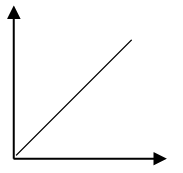
As an example, below is a graph of acceleration versus force applied to an object.

Why use linear regression?

Linear regression is preferable to simply substituting a data pair into an equation and solving for unknowns because:

• a gradient measures the relative changes in each variable, and not at their absolute values – this reduces the effects of systematic errors.

• a gradient is like an average ratio between the dependent and independent variables – this reduces the effects of random errors.

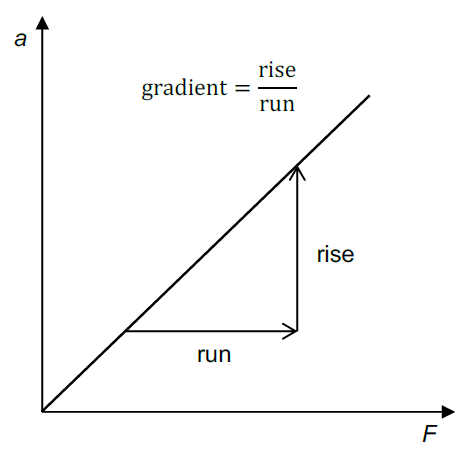
We know of a relationship between force and acceleration, given by Newton’s second law, . We could

rewrite this equation like this:

a = 1 F

m

Y = A X + B

We can see the variables and values that correspond with those in the general equation for a straight line.

When acceleration is the Y-variable and force is the X-variable, then the gradient is equal to and there is

not expected to be a Y-intercept.

If you can calculate the gradient, then you can determine or verify the mass of the object.

Methods for drawing a line of best fit by hand

Data is always affected by experimental error. That is why, even though theory would expect a straight-line graph, the data rarely lies on one. The aim of drawing a line of best fit is to estimate what the line would be, if it were not for the errors. You can do this by hand, but there are computer applications that can do this quite effectively (such as spreadsheets).

Using an ellipse

Draw an ellipse around all the data points, and then draw a line that bisects this ellipse, lengthways.

Just eyeballing it

Line up your ruler along the plotted data points and wiggle it around until you have a line that follows the trend down the middle. The data points should be roughly evenly distributed either side of the line. (technique suggested at MHS)

Importantly, do not force your line so that it goes through the origin. A non-zero Y-intercept, even when you don’t expect one, can sometimes be an important piece of information – it can be an indicator of systematic error, for example.

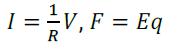
Question 1

Rearrange the equations into the linear form shown by these graphs.

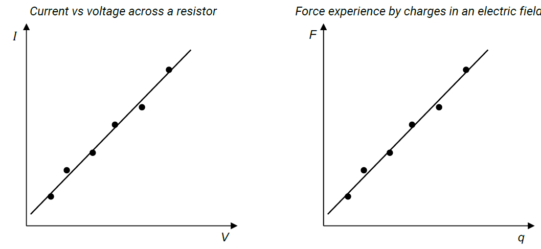
V = IR →

E = F →

q

Question 2

1. Plot the following data on the grid and draw a line of best fit.

Coil current and magnetic field strength inside a solenoid

Magnetic field strength vs coil current inside a solenoid

1.0

0.9

0.8

We don't put the top row above our data tables at MHS...

Magnetic field strength (T)

0.7

0.6

0.5

0.4

0.3

0.2

0.1

0 0 0.2 0.4 0.6 0.8 1.0 1.2

Current (A)

11

1. The equation that relates the magnetic field strength (B) and coil current (I) in this solenoid is

B = 𝜇I

where 𝜇 is a magnetic permeability constant – a measure of the resistance of a material (such as one placed inside the solenoid) against the formation of a magnetic field.

Given that the equation of a straight line is Y = AX + B, identify the term in the equation that represents the:

1. Calculate the gradient of the line of best fit.

Question 3

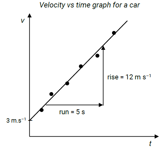
1. The equation of motion relevant to the graph on the left is v = u + at. Rearrange this equation so that it matches the straight-line equation.

2. What does the gradient of this graph represent? Calculate this value.

3. What does the Y-intercept of the graph represent? Write down this value.

4B – Advanced linear regression

Many physical relationships are not linear, but we can still use the techniques of linear regression to establish or verify those relationships. We can linearise non-linear relationships.

By way of example, let’s look at the displacement of an object as it accelerates uniformly with time:

A graph of displacement against the raw time data (below, left) is not linear – in fact, it is parabolic. Displacement is not proportional to time.

Displacement vs time Displacement vs time-squared

If we reinterpret the original equation, realise that we can say displacement is proportional to the square of time (s ∝ t^#). We can reframe the equation like this:

1

s = 2 a t²

Y = A X + B

This tells us to plot displacement s on the Y-axis and time-squared t² on the X-axis – we must square each value of time before we plot it. This graph (above, right) will give us a straight line.

The gradient of the displacement versus time-squared graph is equivalent to # a, or half the acceleration.

"

Thus:

13

so

Question 1

The table below shows the kinetic energy of an object at different speeds.

Kinetic energy of an object at different speeds

Again, we don't put the top row above our data tables at MHS...

• Given that the equation that relates kinetic energy and speed is

rearrange this equation to make it fit Y = AX + B.

• Using your equation in (a), determine the variables that you should graph so that you can get a straight line.

• If you need to process the data for one of the variables so that you can obtain a straight line, do this. Write the new variable name and values in the Processed data column of the table.

  • Identify the quantity that you can determine from the gradient of this graph. Write an equation involving the gradient that you can use to calculate this quantity.

  • Do you expect there to be a Y-intercept? Why or why not?

  • Plot the data from the previous page so that you get a straight-line graph.

Kinetic energy and speed for an object

10.0

9.0

8.0

_

7.0

6.0

5.0

4.0

3.0

2.0

1.0

0

0 0.2 0.4 0.6 0.8 1.0 1.2

• Use the graph to calculate the mass of the object used in the experiment.

Question 2

Waves on the water with a constant speed v were observed – their frequencies and their wavelengths were measured. The equation that relates wavelength and frequency is v = f𝜆.

The graph below, left, shows the relationship between frequency and wavelength.

Wavelength vs frequency for water waves Title:

1. Rearrange the formula so that it is in the form Y = AX + B. (Hint: The Y-variable is a term that involves λ, and the X-variable is a term that involves f).

2. Using your equation in (a), determine the variables that you would graph to obtain a straight line. You can use your answers here to label the graph axes in the graph above, right.

1. What quantity does the gradient of the straight line represent?

Question 3

For each experiment that has been described, think about how you would graph the variables that have been mentioned.

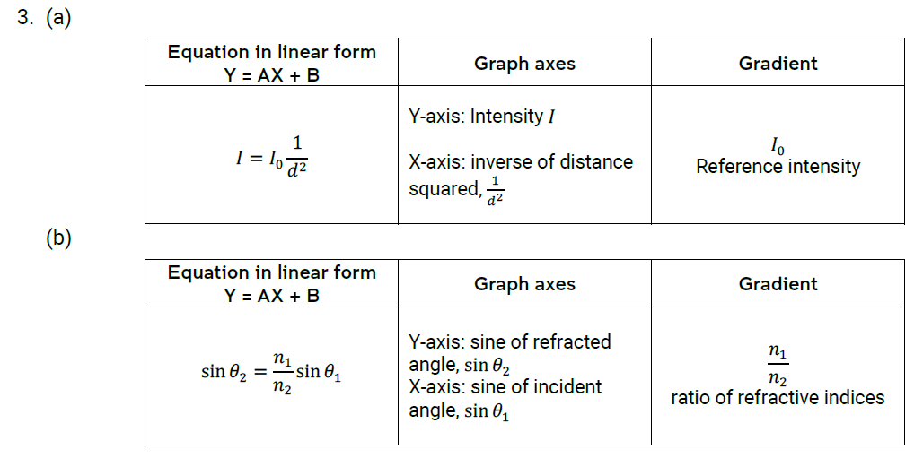
Rewrite the equations in linear form, determine and label the graph axes, and write down the terms corresponding to the line’s gradient.

1. You measure the intensity of light I at several distances from a lamp, d. We know that the intensity of light decreases with distance by the inverse square law:

"

where is the reference intensity of light (taken at d = 1 m).

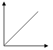
1. You point a laser at a glass block, and you measure the incident angle 𝜽₁ and refracted angle 𝜽₂. We know the angles are related by Snell’s law:

where and are the refractive indices of the air and the glass respectively.

– Accuracy and error

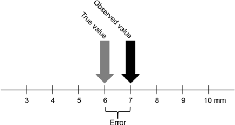Accuracy is the closeness of an observed value to its “true” value (a true value could be some theoretical value, or a value accepted by physicists and tabulated in secondary sources).

On some level, every measurement is limited in its accuracy. One reason is that there are limitations in the instruments we use for measuring – they may lack sensitivity, or the graduations on them might not be fine enough (their resolution).

Environmental factors can also interfere with making measurements, and we as humans have our limitations in making and reading measurements, too.

The difference between an observed value and its true value is called error (for us, it does not mean “mistake”, as is its common meaning).

There are three ways that we can quantify error and accuracy:

High accuracy measurements have small errors, and low accuracy measurements have large errors. You could set an arbitrary limit on what you call “accurate”, say for example, “less than 5% error”.

We did not use the absolute error or accuracy concepts shown above in the MHS

Question 1

Booklet but relatively easy concept to follow...

Calculate the absolute and percentage errors for the following results. Using the arbitrary criteria for accuracy as being >95% accurate, assess whether the results are accurate or inaccurate.

18

Systematic and random errors

When you make multiple measurements and compute the errors, you might start to recognise patterns n how and when they occur. Because of this, errors can be put into one of two categories depending on how they behave:

• Systematic errors –When repeated, observed values are displaced in same direction from the true value. That is, the observed values might read consistently higher or consistently lower than the true value.

These types of errors are often caused by improperly calibrated measuring instruments, or “zero” errors (such as when an electronic balance shows a non-zero reading when there is nothing on its pan – every reading will be higher than it should be).

• Random errors – When repeated, observed values are scattered randomly above and below the true value.

These types of errors are often caused by random fluctuations in the ambient conditions or uncontrolled variables.

Systematic errors shift all measurements in the same direction.

Random errors cause measurements to spread randomly in all directions.

Question 2

Assess whether the following situations represent systematic or random errors.

1. The Royal Australian Mint states that the mass of a 50-cent coin is 15.55 g, so some students choose to measure some for themselves. First, they measure the mass of one coin, and then of two coins, and so on.

Predict the “true” values and compare them with the observations.

What type of error is demonstrated here?

1. Some students are interested in the boiling temperature of water. They go away in groups and heat equal amounts of water drawn from the same laboratory tap. They measure the water temperature with thermometers once boiling. Below are their results.

What type of error is demonstrated here?

Improving accuracy (that is, reducing errors!)

To increase accuracy, we therefore need to reduce error. We can do that by modifying experimental techniques or procedures to make the error absolutely smaller, or by making the error smaller relative to the value we are measuring.

Question 3

How does the use of measuring instruments with appropriate sensitivity and resolution improve accuracy?

Question 4

The following procedure reduces the relative error of a measurement:

• Instead of measuring the relatively quick period of a short pendulum, you could measure the relatively slow period for a long pendulum.

Explain how this sort of technique improves accuracy.

Question 5

Explain how pressing the “tare” (or “zero”) button on an electronic balance before measuring a mass reduces systematic error. What might happen if you did not press the tare button?

Question 6

Explain how taking measurements in a series of repeated trials, and then calculating an average, reduces random error.

– Estimating uncertainties in measurements

While the concept of error compares measurements against values assumed to be “true”, there are many more measurements that cannot be compared to known or accepted values. For example, if I measured the length of a bit of string that I have, what is my error? I cannot compare my measurement with that of an expert – they don’t have my string!

Instead, what we should do is report our measurements with some indication of the certainty we have in it.

Remember, every measurement we make is, on some level, an approximation. To communicate how accurate we think our measurement is, we can cite a margin of error which we call uncertainty.

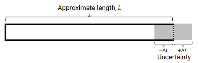
If we have a measurement x, then the uncertainty in that measurement is Δx. When we communicate the measurement to others, we write it in the form x ± ∆x. The uncertainty has the same units as the measurement.

For example, the bar in the diagram above could have length 6.0 ± 0.5 cm.

So, when we make measurements, how do we know how big our uncertainty is? Well, we will answer that in this unit.

Question 1

What is the length and uncertainty of the bar below?

7.0 cm

0.3 cm 0.3 cm

Length =

A smaller uncertainty means that we can have higher confidence in a measurement. Compare this bar to the one earlier, in the notes (L = 6.0 ± 0.5 cm). Which measurement can we have more confidence in?

21

Writing uncertainties

Recall how significant figures communicate the uncertainty in a number. For example, 1234 m (4 significant figures, has uncertainty ±0.5 m) has less uncertainty than 1200 m (2 significant figures, has uncertainty

±50 m). Because of this, there is a link between the number of digits that we report for a measurement and its uncertainty.

So, to properly present a number with its uncertainty:

• Step 1: Round the uncertainty to one significant figure.

• Step 2: Round the measurement to the same place value (decimal place).

If the measurement’s and uncertainty’s lowest place values don’t match, then the extra digits are meaningless – a relatively large uncertainty swamps the small value added by the extra digits.

Examples:

• 9.61482 ± 0.0372 m s^–2 should be rounded to 9.61 ± 0.03 m s^–2

• 1522.1 ± 68.34 km should be rounded to 1520 ± 70 km

Question 2

Rewrite these uncertain quantities with the appropriate digits.

Just like with errors, we can express uncertainties in absolute terms, or in relative terms.

Δx

x

Relative uncertainty

(also called percentage uncertainty when expressed as %)

Δx

Absolute uncertainty

(has the same units as the measurement)

For example, the resistance of an electrical component could be written in absolute terms as 12.2 ± 0.3 Ω or in percentage terms as 12.2 Ω ± 2%

We removed percentage uncertainties from the 2022 skills booklet...

Question 3

Compute the percentage uncertainties in the following values.

How big should my uncertainty be?

There is no single way to estimate the uncertainty in a measurement – it depends on how you have made your measurement. Next, we will focus on the uncertainty in a single direct measurement, and then the uncertainty in an average from repeated trials.

– Uncertainty in direct measurements

The uncertainty in a direct measurement comes from our ability to make readings with measuring instruments.

Some measuring instruments are labelled with the accuracy or uncertainty that you can expect when you use them. In this case,

Digital Caliper Resolution: 0.01 mm

Accuracy: ±0.02 mm

±0.02 mm.

For all other instruments, the absolute smallest uncertainty they provide is limited by the graduations marked on them – this is known as the limit of reading:

Bar

This ruler is graduated in 1.0 cm increments. The uncertainty in direct measurements made with this ruler would be ±0.5 cm.

In the diagram above, we can read that the bar is near to 3.0 cm (the nearest centimetre mark) but we cannot confidently estimate the length of the bar any finer than that.

We would report this measurement as 3.0 ± 0.5 cm (notice the “.0” in the measurement – so that the number of decimal places in the uncertainty matches).

Question 4

1. What is the smallest uncertainty that you can expect with these instruments?

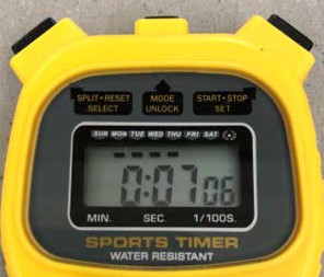
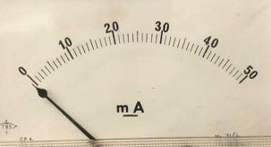
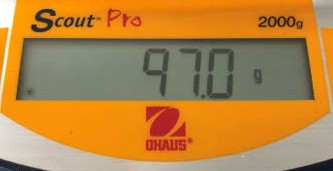
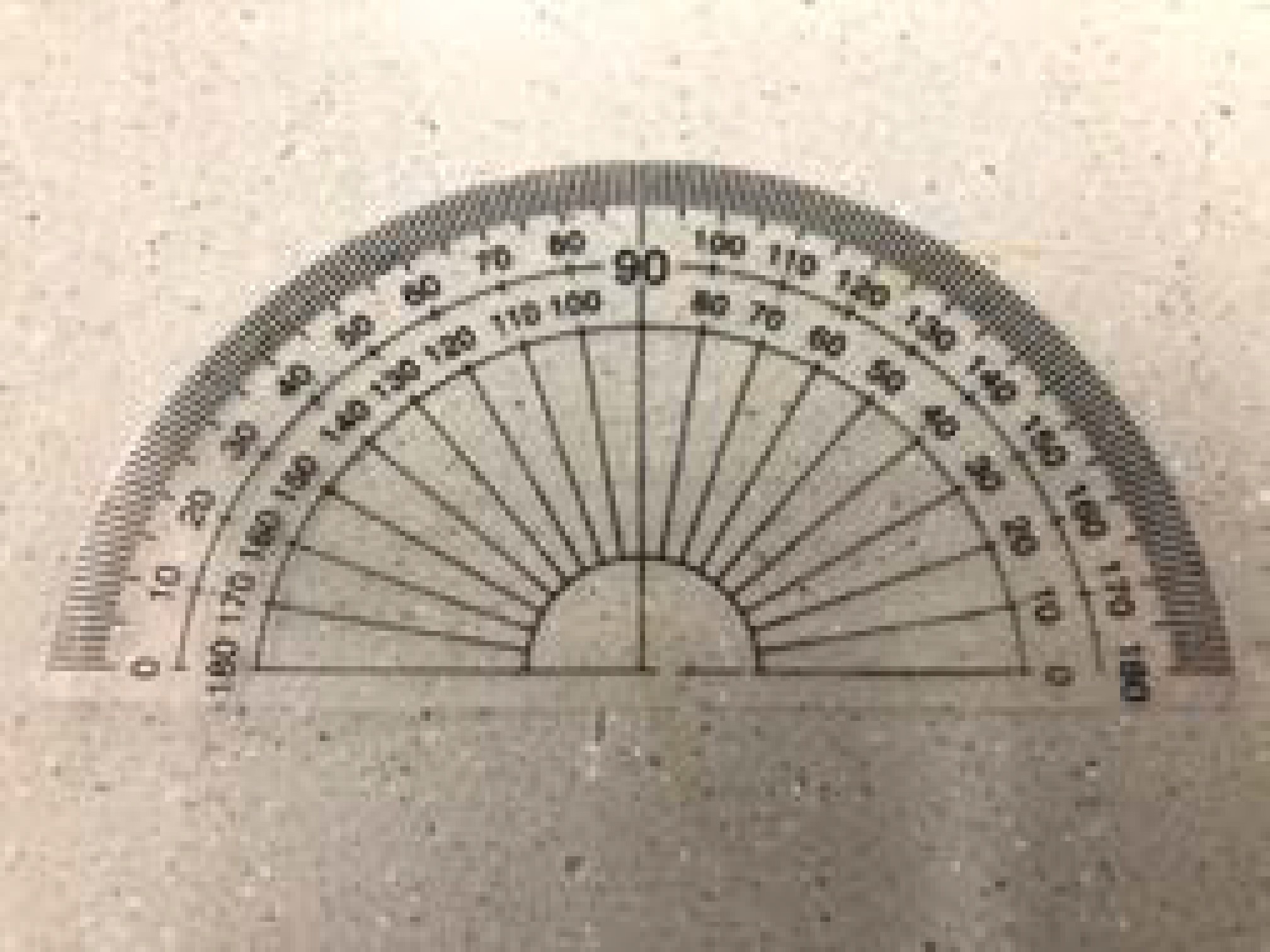
Stopwatch Milliammeter Electronic balance Protractor

1. For the stopwatch and the electronic balance, write the reading and its uncertainty with the appropriate number of digits.

23

– Estimating larger uncertainties in direct measurements

Sometimes the markings on an instrument cannot be confidently read by us and the uncertainty is actually larger. For example, imagine you are attempting to measure the bounce height of a ball. The ball moves so quickly that you cannot precisely measure to millimetre accuracy on the adjacent ruler.

In cases like this, you will have to use your judgement – perhaps you are only confident that you can measure to the nearest 5 cm, so your uncertainty is half of this, ±2.5 cm.

This practice does rely on some subjectivity. If you are unsure, it is always preferable to overestimate your uncertainty than to dishonestly claim that it is smaller.

– Uncertainty in an average of trials

Recall that conducting repeated trials and then computing an average helps to reduce random error. While we can assume that the average is more accurate than any of the trials, there is still some uncertainty in the average.

At MHS. we use the technique of calculating the average and then using the largest deviation in the measurement form the average value as our uncertainty.

Question 5

Determine the average and uncertainty from the following sets of measurement trials.

– Assessing reliability in experiments

Reliability refers to the consistency in results – repetition returns results that lie within a small margin of error. There are two ways of looking at reliability:

• Internal reliability is when repeated trials within an experiment are consistent. This is sometimes also called precision.

  • External reliability is when the results from one experiment are consistent with those from other experiments that are conducted the same way.

NOTE – we did not use these terms in the MHS skills booklet…

When assessing reliability, sometimes it is enough to make broad subjective judgements (for example, “overall, the results appear to be roughly consistent”) but it is preferable to fall back on some kind of quantitative basis.

Evaluating reliability

One way to assess reliability might be to quantify the spread of trials around an average – large spreads are unreliable, and smaller spreads are reliable.

Data from reliable trials are clustered closely.

Data from unreliable trials are much more spread out.

We could judge a set of trials to be reliable if the relative uncertainty of the trials is less than some arbitrary limit, say, less than 5%.

For example, the following measurements of the same resistor were collected. The average is shown, and the uncertainty was calculated using:

Uncertainty = ± largest deviation from average value

This allows us to calculate the percentage of uncertainty of this data set as or 6%. According to our criteria, these trials are not reliable.

Perhaps it might be better to say that they have low reliability.

Question 1

A physics class is set the task of measuring acceleration due to gravity, g, using pendulums. They go away in groups to do this, and when they have completed their experiments, they return to report their findings. Below are their results.

Physics class results – acceleration due to gravity, g

1. Which concept is being demonstrated here? Internal or external reliability?

2. Calculate the average and its uncertainty for this set of data.

3. Assess the reliability of this set of data.

Question 2

Another physics class is investigating the stopping distance of a bicycle from different speeds. A student rides the bike at a designated speed and applies the brakes once it passes a mark on the ground. The remaining students measure the distance to where the bike has stopped. The students conducted 5 trials for every speed. Below is one set of their trials.

Physics class results – Stopping distances at 10 km/h

1. Which concept is being demonstrated here? Internal or external reliability?

2. Calculate the average and its uncertainty for this set of data.

3. Assess the reliability of this set of data.

Question 3

(a) Can simply repeating a measurement or an experiment on its own improve reliability? Why/why not?

Question 4

1. It can be said that variability is the enemy of reliability. What does this mean?

2. What is the cause of variability, and how can it be minimised?

– Assessing validity in experiments

A valid experiment is one that examines what is intended – the relationship between an independent variable and a dependent variable with minimal interference from other factors. These other factors might be the variables that we should control (hold constant), or the level of care with which we conduct the experiment and make measurements.

If we only vary the independent variable and keep all the other variables the same, then we can be confident that the effects that we observe are due only to the changes that we have made. We can say that the experiment is valid.

However, if we do not keep the other variables the same, then we cannot be certain that our observations are only due to the independent variable. This would mean that the experiment would be invalid.

If we are careless when we conduct experiments, make inaccurate measurements, or use inappropriate equipment, then his also invalidates the experiment.

Question 1

Some students wish to investigate the effect of a force on accelerating toy cars.

They hypothesise that increasing the force on the cars will proportionally increase their rates of acceleration because of the equation

They test their hypothesis with a range of toy cars. Below is the data that they collected.

1. What was the independent variable?

2. What was the dependent variable?

3. Does the data show a proportional relationship between force and acceleration, as predicted by the students?

4. Based on this data alone, what can the students conclude about their hypothesis?

Later, the teacher who was observing the students made some related measurements of her own. Her data is displayed below.

1. Can we confidently attribute the acceleration of the cars purely to the force applied? What does this mean for our trust in the students’ conclusions in part (d)?

2. Write a short paragraph that assesses the validity of the students’ investigation.

3. How can the validity of the experiment be improved?

Question 2

What are the conditions for a valid experiment?

Solutions

– Units for measurement

1. mass – kilogram, amount of substance – mole, electric current – ampere, luminous intensity – candela, time – second, thermodynamic temperature – Kelvin, length – metre.

2. m s^-2 kg m s^-2 m² m³ kg m s^-2

3. joule (J), coulomb (C), hertz (Hz), pascal (Pa), volt (V).

4. (a) 58.3 MN, 7.48 µA, 101.3 kPa

(b) 0.000 000 576 m, 450 000 N, 0.000 916 A

5. 1 mg, 1 g, 1 tonne, 1 kilotonne

– Significant figures

1. 3, 2, 5

3, 4, 6

2. 81 100 m 2.146 × 10⁶ kg

618 000 K 0.00571 C

8.0 s 160 W 3. ±0.5 m ±0.05 A

±0.005 kg ±0.0005 N

4. (a) 1.7 m s^–2

(b) 137 m

5. (a) 22.84 kg

(b) 900.0 m

– Scientific notation and orders of magnitude

1. 15 000 N 0.003145 J

0.00000915 m 7 200 000 000 V

2. 9.22 × 10³ m s^–1 3.25 × 10^–4 C

1.27 × 10^–1 A 7.23 × 10⁶ m²

1. Order of magnitude: 7, - 3

-3, 7

1. 2 orders of magnitude, 2 orders of magnitude 2 orders of magnitude, 3 orders of magnitude

4A – Linear regression

1.

2. (a)

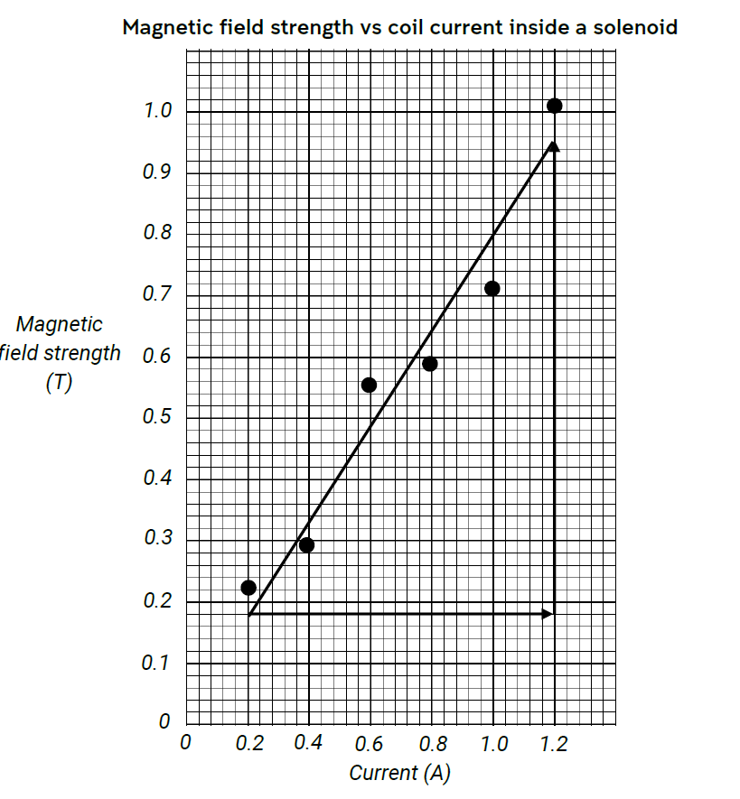
(b) Y-variable – Magnetic field strength, B X-variable – Current, I

Gradient – Magnetic permeability constant, µ Y-intercept – None

(c)

3. (a) v = at + u

1. acceleration, 2.4 m s^–2

2. initial speed, 3 m s^–1

4B – Advanced linear regression

1. (a)

(b) Y-variable – kinetic energy, K

X-variable – velocity-squared, v²

(c)

1. gradient = ½ m

2. No, we should not expect a Y-intercept. There was no ‘B’ term when we put the equation into a straight-line form.

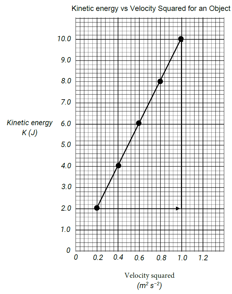
(g)

2. (a)

1. Y-variable – wavelength, λ

X-variable – inverse of frequency,

Gradient = velocity, v

– Accuracy and error

1.

2. (a)

This is a demonstration of systematic error.

(b) The values vary randomly around 100° C – it is a demonstration of random error.

1. Sensitive measuring instruments respond appropriately to variances in quantities being measured, meaning that it is more likely that a measurement will be close to the true value. Using measuring instruments of appropriate resolution means that a measurement is more likely to be made close its true value with a small uncertainty.

2. This technique improves accuracy by increasing the size of the observation relative to the error. The timing errors introduced by using a stopwatch stay about the same in absolute terms (~0.5 seconds), but by increasing the length of the observation, the error becomes a smaller fraction.

3. Taring an electronic balance ensures that it reads zero when there is nothing placed on it. If the balance was not tared, then there is a possibility that every reading made will be offset from their actual values.

4. Random errors cause values to vary randomly above and below a true value, in roughly even proportions. A technique like averaging seeks the middle, so an average is likely to approach the true value.

– Estimating uncertainty in measurements

1. 7.0 ± 0.3 cm – We can have more confidence in this measurement. 2. 51.78 ± 0.08 m 0.287 ± 0.005 A

841 100 ± 500 kg (6.3 ±0.5) × 10⁴ V

3. 1% 3%

14% 3%

4. (a) ±0.01 seconds, ±0.5 mA, ±0.1 g, ±0.5°

(b) 7.06 ± 0.01 seconds, 97.0 ± 0.1 g

5. 9.41 ± 0.71 so this is recorded as 9.4 ± 0.7 m s^–2, 76.52 ± 3.71 so 77 ± 4 mL, 100.24 ± 0.07 Ω

– Assessing reliability in experiments

1. (a) External reliability, (b) 10 ± 1 m s^–2, (c) 10 % relative uncertainty – low reliability.

2. (a) Internal reliability, (b) 6.2 ± 0.2 m, (c) 3% relative uncertainty – high reliability.

3. Simple repetition of measurements or experiments do not on their own improve reliability. If nothing has been done to address the causes of variability in the data, then repetitions may just continue showing the variations that are markers of unreliability.

4. (a) Reliability means that measurements or experiments return very similar results every time they are repeated, that is, there is minimal variation between each result. If there is a lot of variation, then results are not reliable.

(b) Variability is caused by sources of random error. These could be uncontrolled variables or influences from environmental conditions that cause random fluctuations. They could also come from sloppy work. Variability can be reduced by controlling variables, taking many trials and finding averages, and reducing relative random errors.

(Note that sources of systematic errors do not affect reliability – these errors usually affect measurements in a set of trials the same way, e.g. shifting them all in one direction, rather than causing then to vary randomly – it is possible to have inaccurate yet reliable results because of this)

– Assessing validity in experiments

1. (a) Independent variable – Force

2. Dependent variable – Acceleration

3. The data does not show a proportional relationship between force and acceleration.

4. Based on this data, the students might conclude that their hypothesis was false.

5. The teacher’s data shows that they did not control the masses of the cars. This means that we cannot trust the conclusion in (d).

6. The student’s investigation was not valid because they did not control all variables.

7. The validity could be improved by controlling the mass of the toy cars, i.e. keeping them all the same mass.

8. The designed experiment must answer our aim by being a fair test. In a valid experiment, only the independent variable should be varied; all other variables should be controlled (held constant). Also, the equipment used when conducting the experiment must be appropriately chosen, and measurements should made carefully with instruments of appropriate type and resolution.

References

First Year Physics Unit 2020, First year physics laboratory manual, PHYS 1121: Physics 1A, PHYS1131: Higher Physics 1A, University of New South Wales, Sydney.

Masons, C., Burns, A., Nair, S. 2019, Evaluating Scientific Data, NSW Department of Education, accessed 16 January 2020, https://schoolsequella.det.nsw.edu.au/file/ee66cc99-c090-42d7-8bc8- 85734c19a0b9/1/Evaluating_data.docx

NSW Department of Education 2018, Guidelines for some working scientifically skills, accessed 16 January 2020, https://schoolsequella.det.nsw.edu.au/file/bde20be7-b530-44ee-b8da-ba794fa4fca6/1/working- scientifically-skills-guidelines.docx

NSW Education Standards Authority 2017, Physics stage 6 syllabus, NSW Education Standards Authority, Sydney.