Chapter 4: Discrete Random Variables
Introduction
- Random Variable Notation: Upper case letters such as X or Y denote a random variable. Lowercase letters like x or y denote the value of a random variable
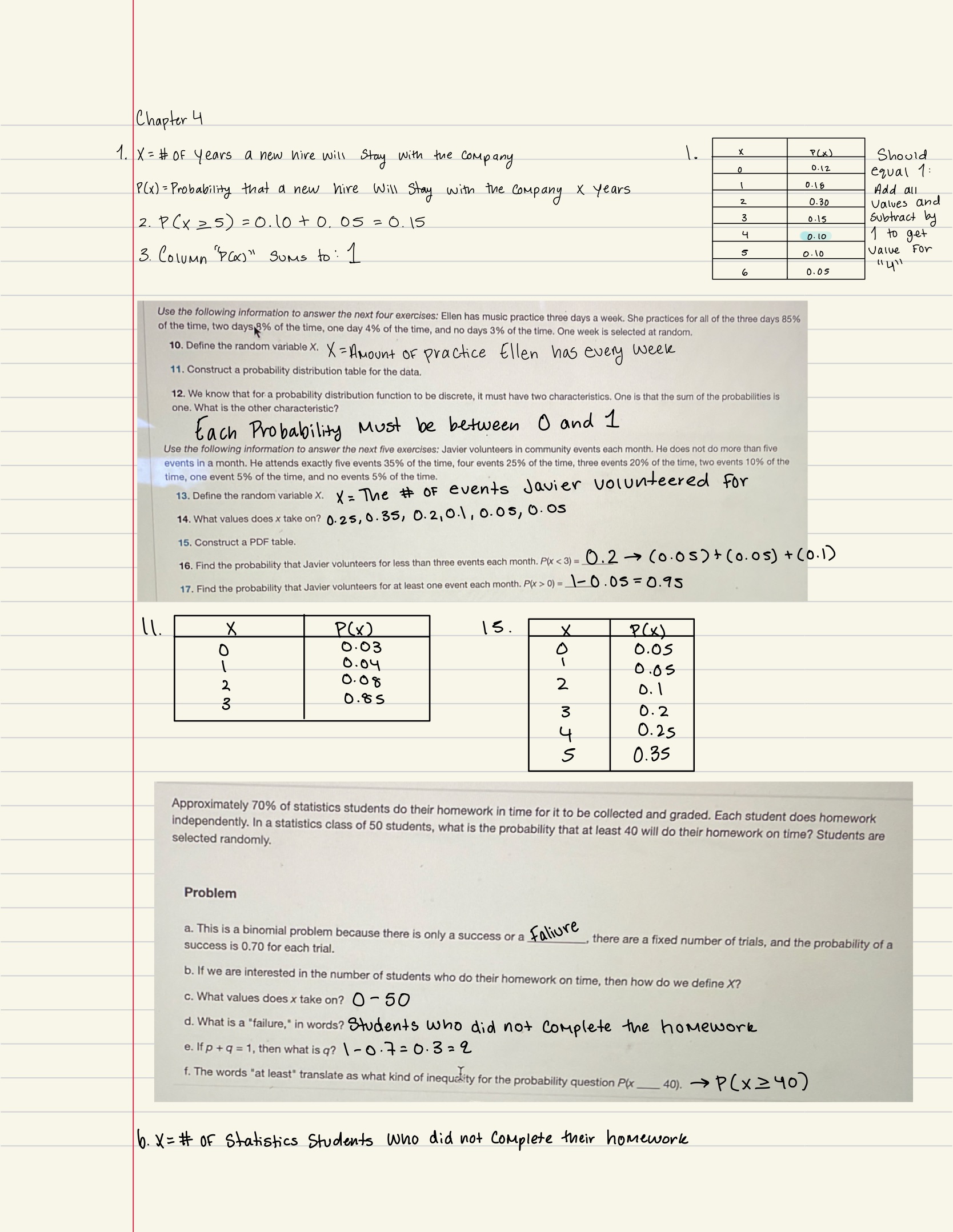
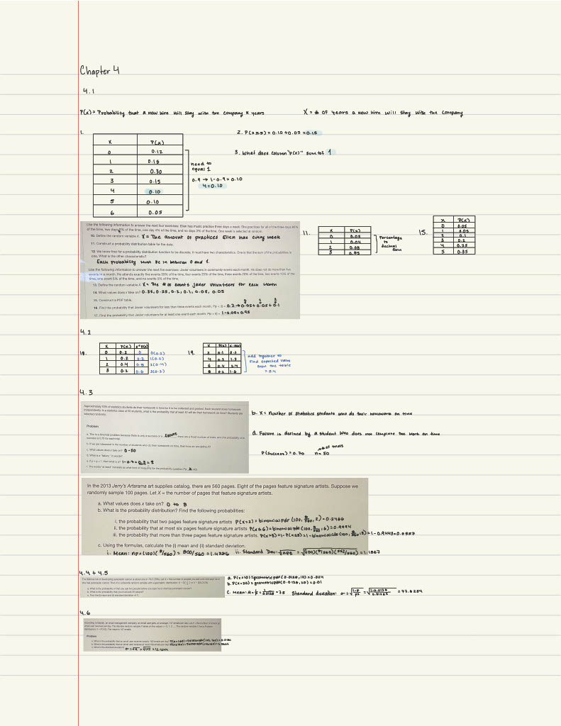
4.1 Probability Distribution Function (PDF) for a Discrete Random Variable
- A discrete probability distribution function has two characteristics:
- Each probability is between zero and one, inclusive.
- The sum of the probabilities is one.
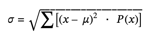
4.2 Mean or Expected Value and Standard Deviation
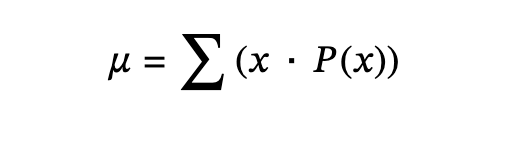
- Expected value: Referred to as the long-term average or mean. This means that over the long term of doing an experiment over and over, you would expect this average.
- The Law of Large Numbers: as the number of trials in a probability experiment increases, the difference between the theoretical probability of an event and the relative frequency approaches zero
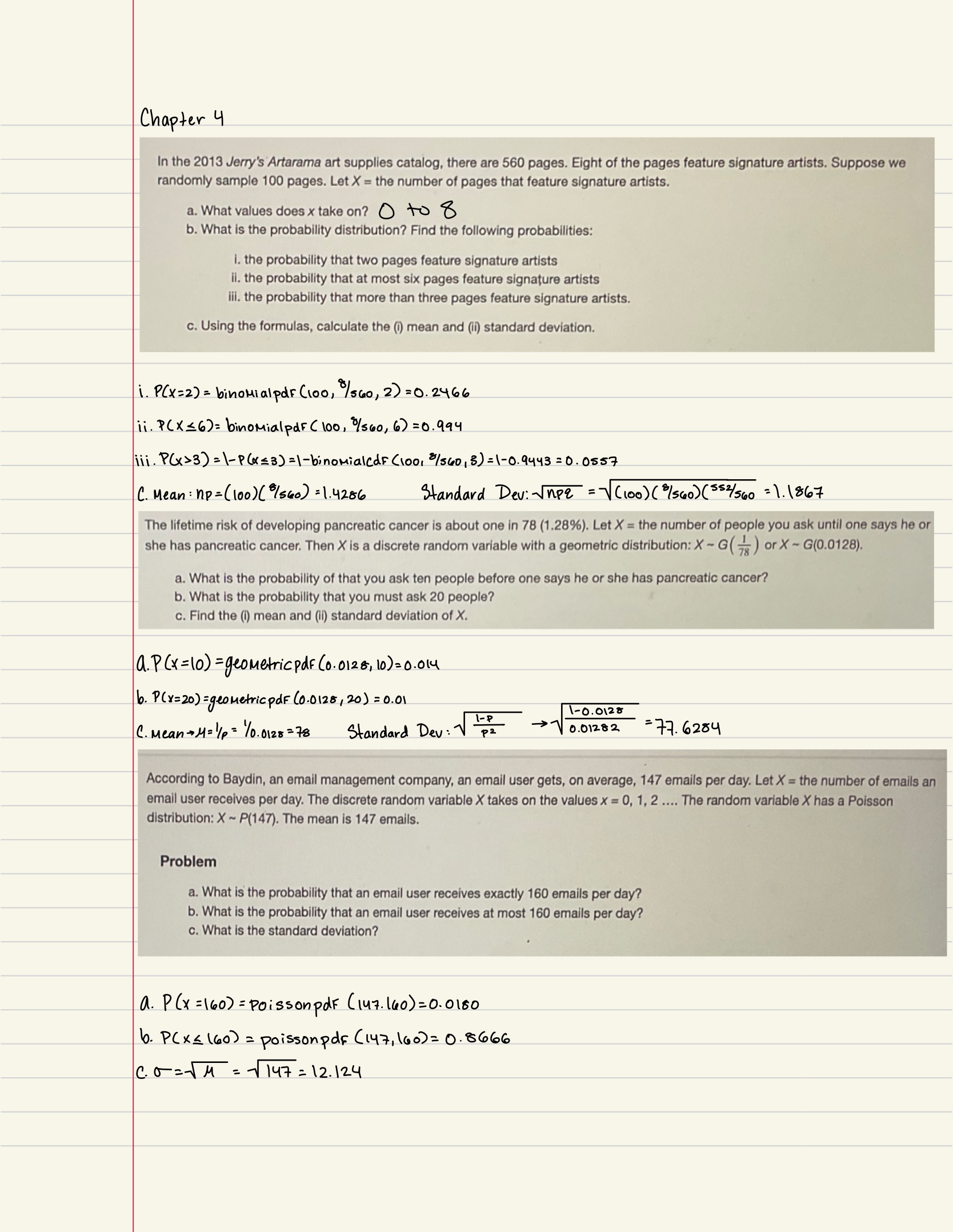
4.3 Binomial Distribution
- 3 Characteristics of a binomial experiment
- There are a fixed number of trials
- There are only 2 possible outcomes
- The n trials are independent and are repeated using identical conditions
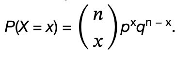
- Binomial probability distribution:
- Mean→μ = np
- Variance→σ2 = npq
- Standard deviation→ σ = √npq.
- Bernoulli Trial: There are only two possible outcomes called “success” and “failure” for each trial. The probability p of a success is the same for any trial (so the probability q = 1 − p of a failure is the same for any trial).
Notation for the Binomial: B = Binomial Probability Distribution Function
- X ~ B(n,p): Read this as "X is a random variable with a binomial distribution." The parameters are n and p; n = a number of trials, and p = probability of success on each trial.
- Mean→μ = np
- Standard deviation→σ = √npq
4.4 Geometric Distribution
- 3 Characteristics of a geometric experiment
- There are one or more Bernoulli trials with all failures except the last one, which is a success. In other words, you keep repeating what you are doing until the first success.
- In theory, the number of trials could go on forever. There must be at least one trial.
- The probability, p, of a success and the probability, q, of a failure is the same for each trial. p + q = 1 and q = 1 − p.
- X = the number of independent trials until the first success
Notation for the Geometric: G = Geometric Probability Distribution Function
- X ~ G(p): Read this as "X is a random variable with a geometric distribution." The parameter is p; p = the probability of success for each trial.
- Mean→μ = 1/p
- Standard Deviation→σ = √1/𝑝(1/𝑝−1)
4.5 Hypergeometric Distribution
- 5 Characteristics of a hypergeometric experiment
- You take samples from two groups.
- You are concerned with a group of interest, called the first group.
- You sample without replacement from the combined groups.
- Each pick is not independent, since sampling is without replacement.
- You are not dealing with Bernoulli Trials.
- X = the number of items from the group of interest.
Notation for the Hypergeometric: H = Hypergeometric Probability Distribution Function
- X ~ H(r, b, n): Read this as "X is a random variable with a hypergeometric distribution." The parameters are r, b, and n; r = the size of the group of interest (first group), b = the size of the second group, and n = the size of the chosen sample.
4.6 Poisson Distribution
- 2 Characteristics of a Poisson experiment
- Gives the probability of a number of events occurring in a fixed interval of time or space if these events happen with a known average rate and independently of the time since the last event.
- May be used to approximate the binomial if the probability of success is "small" (such as 0.01) and the number of trials is "large" (such as 1,000).
- X = the number of occurrences in the interval of interest.
Notation for the Poisson: P = Poisson Probability Distribution Function
- X ~ P(μ): Read this as "X is a random variable with a Poisson distribution." The parameter is μ (or λ); μ (or λ) = the mean for the interval of interest. The standard deviation of the Poisson distribution with mean µ is Σ=√μ
Example