Chapter 6: The Normal Distribution

6.1 The Standard Normal Distribution

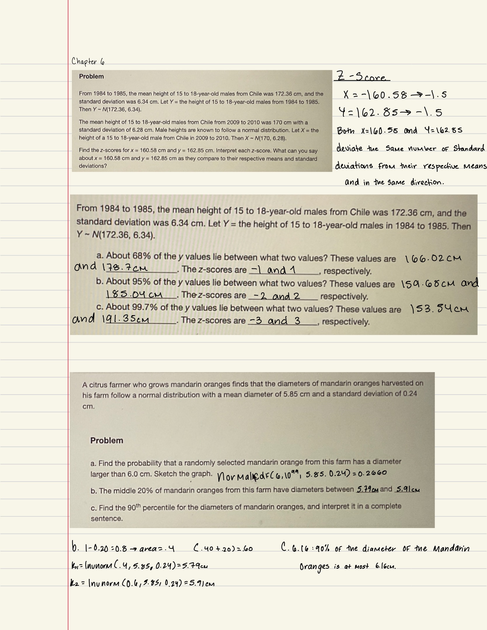
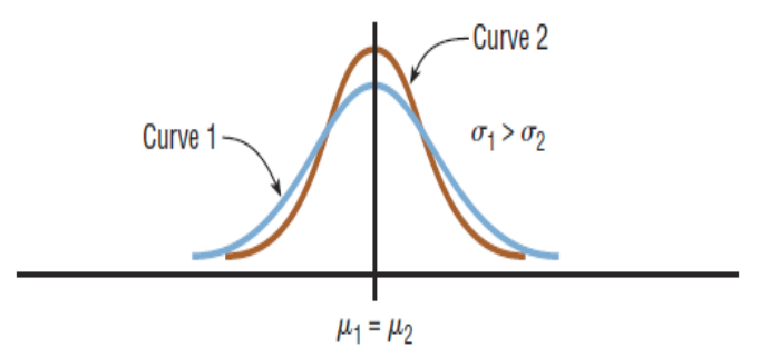
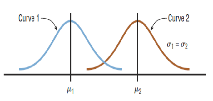
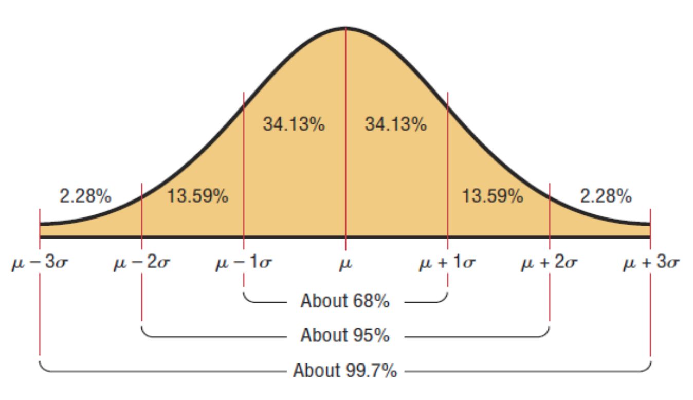
• Normal distribution: A bell curve or a Gaussian distribution curve. If a random variable has a probability distribution whose graph is continuous, symmetric, and bell-shaped.

• Approximately normally distributed variables: Many continuous variables (e.g. weights, heights) have distributions that are bell-shaped

• Standard normal distribution: a normal distribution with a mean of µ = 0 and a standard deviation of σ = 1.

• Z-score formula: X − 𝝁 / σ

  

  

  

Summary of the Properties of the Theoretical Normal Distribution

• Mean = Median = Mode

• A normal distribution curve is unimodal.

• The curve never touches the x-axis.

• The total area under a normal distribution curve is equal to 1.00

  

6.2 Using the Normal Distribution

• Normal Distribution: X ~ N(µ, σ) where µ is the mean and σ is the standard deviation.
• (P → X): X = 𝝁 + 𝝈Z
• Number of units (individual/items) satisfying a condition→ Total number of units given in the problem × are calculated based on condition
• Calculator function for probability: normalcdf (lower x value of the area, upper x value of the area, mean, standard deviation)
• Calculator function for the kth percentile: k = invNorm (area to the left of k, mean, standard deviation)

6.3 The Central Limit Theorem

• Sampling distribution of sample means: a distribution using the means computed from all possible random samples of a specific size taken from a population.
• Sampling error: the difference between the sample measure and the corresponding population measure because the sample is not a perfect representation of the population.

Properties of the Distribution of Sample Means

• The mean of the sample means = population mean.
• The standard deviation of the sample means < standard deviation of the population
• The standard deviation of the sample means will be equal to the population standard deviation divided by the square root of the sample size.
• The Central Limit Theorem: sample size n, mean µ, and standard deviation σ are given
• Standard error of the sample mean: 𝝈/ √n

Examples

\
\
\