Chapter 4: Probability, Sampling, and Distributions

4.1 Probability

Probability: refers to the likelihood of a particular event of interest occurring

• To calculate the probability of an event occurring, we simply divide the number of occurrences of the desired outcomes by the total number of possible outcomes.

Example: tossing a coin with one desired outcome (heads) and two possible outcomes (heads or tails) = 1 ÷ 2 = 0.5 [in percentage = 0.5 * 100 = 50%]

4.1.1 Conditional Probabilities

Conditional Probability: the probability of a particular event happening if another event (or set of conditions) has also happened)

4.1.2 Applying Probabilities to Data Analyses: Inferential Statistics

Inferential Statistics: techniques employed to draw conclusions from your data.

• From the data, we would try to make some inferences about the relationship between the two variables in the population.
• It is possible that we may draw the wrong conclusions from our statistical analyses because the statistical techniques we use in order to draw conclusions about underlying populations are based upon probabilities; therefore, we need to be constantly aware of the fallibility of such techniques.

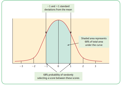
4.2 The Standard Normal Distribution

Standard Normal Distribution (SND): the distribution of z-scores; normally shaped probability distribution which has a mean (as well as median and mode) of zero and a standard deviation of 1

• In order to use the standard normal distribution for analyzing our data, we often transform the scores in our sample to standard normal scores.
• A useful feature of the SND is that we can use it to calculate the proportion of the population who would score above or below your score.

z-scores: aka standardized scores; you can convert any score from a sample into this by subtracting the sample mean from the score and then dividing by the standard deviation

• z-scores are expressed in standard deviation units: that is, the z-score tells us how many standard deviations above or below the mean our score is.
• If you have a negative z-score then your score is below the mean; if you have a positive z-score then your score is above the mean.

Example:

mean IQ score = 100

IQ standard deviation = 15

your IQ score = 135

z-score = ?

(your IQ score - mean IQ score) ÷ IQ standard deviation = (135 - 100) ÷ 15 = 2.33

• Your score is 2.33 standard deviations above the mean.

Probability Distribution: a mathematical distribution of scores where we know the probabilities associated with the occurrence of every score in the distribution'; we know that the probability is of randomly selecting a particular score or set of scores from the distribution

• Advantage: there is a probability associated with each particular score from the distribution.

• An important characteristic of probability distributions is that the area under the curve between any specified point represents the probability of obtaining scores within those specified points.

  

4.2.1 Comparing Across Populations

Example: You decided to take a course in pottery and weightlifting. At the end of the courses, you were graded 65% for pottery and 45% for weightlifting. Suppose that the mean and standard deviation for pottery are 56% and 9% and for weightlifting 40% and 4%. Which career would be better for you?

z-score for pottery = (65-56) ÷ 9 = 1

z-score for weightlifting = (45-40) ÷ 4 = 1.25

• On the face of it, you might feel justified in pursuing pottery than weightlifting since you scored higher in pottery. However, when you compared yourself to others in your groups, using z-scores, it showed that you were 1 standard deviation above the mean in pottery and 1.25 standard deviation above the mean for weightlifting. Therefore, you are comparatively better at weightlifting compared to pottery based on the z-scores.

4.3 Applying Probability to Research

• One of the simplest ways of applying probabilities to research and of estimating population parameters from sample statistics is to calculate confidence intervals.

4.4 Sampling Distributions

Sampling Distribution: a hypothetical distribution. it is where you have selected an infinite number of samples from a population and calculated a particular statistic (e.g., a mean) for each one; when you plot all these calculated statistics as a frequency histogram, you have a sampling distribution

Sampling Distribution of the Mean: if you plotted the sample means of many samples from one particular population

• An interesting property of sampling distributions is that, if they are plotted from enough samples, they are always approximately normal in shape.
• In general, the larger the samples we take, the nearer to normal the resulting sampling distribution will be.

Central Limit Theorem: states that as the size of the samples we select increases, the nearer to the population mean will be the mean of the sample means and the closer to normal will be the distribution of the sample means

4.5 Confidence Intervals and the Standard Error

Point Estimate: a single figure of an unknown number

Interval Estimate: range within which we think the unknown number will fall

Confidence Interval: a statistically determined interval estimate of a population parameter

• We usually set up 95% confidence intervals and you will find that it is often the case that such intervals can be quite narrow (depending upon the size of your samples).

4.5.1 Standard Error

Standard Error: refers to the standard deviation of a particular sampling distribution; in the context of the sampling distribution of the mean, it is the standard deviation of all of the sample means

• For any given population, the larger the samples we select, the lower the standard error.
• It has been shown that if, for any given example, we divide the standard deviation by the square root of the sample size, we get a good approximation of the standard error.
• Formula: standard deviation of the sample divided by the square root of the sample size
• To work out the 95% confidence interval, we have to multiple the standard error by 1.96.
• Confidence interval is calculated as the mean ± the standard error * 1.96.
• What the confidence interval tells us is that if we were to replicate our study 100 times then in 95 out of those 100 replications the confidence interval we calculate would contain the population mean.

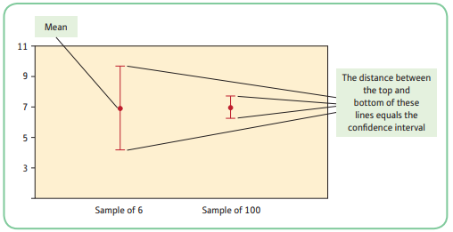
4.6 Error Bar Charts

Error Bar Chart: a graphical representation of confidence intervals around the mean

• Error bar charts simply display your means as a point on a chart and a vertical line through the mean point that represents the confidence interval. The larger the confidence interval, the longer the line is through the mean.

  

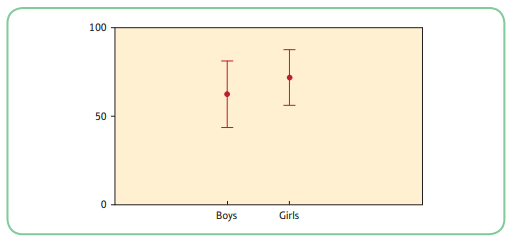
4.7 Overlapping Confidence Intervals

• If there is substantial overlap between the 2 sets of confidence intervals, we cannot be sure whether there is a difference in the population means.

  

• When the confidence intervals do not overlap, we can be 95% confident that both population means fall within the intervals indicated and therefore do not overlap. This would suggest that there is a real difference between the population means.

  

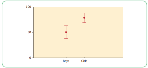
• Examining confidence intervals gives us a fair idea of the pattern of means in the populations.

4.8 Confidence Intervals Around Other Statistics

• We can calculate confidence intervals for a number of different statistics, including the actual size of a difference between two means, correlation coefficients, and t-statistics.
• Where a point estimate exists, it is usually possible to calculate an interval estimate.
• If you are investigating differences between groups, the confidence interval of the magnitude of the difference between the two groups is very useful. If the confidence interval includes zero, it suggests that there is likely to be no difference between your groups in the population.