7.1 Properties of the Normal Distribution
Learning Objectives:
1. Use the uniform probability distribution
2. Graph a normal curve
3. State the properties of the normal curve
4. Explain the role of area in the normal density function
Probability density function (PDF) for a continuous random variable:
A Probability Density Function (PDF) is an equation used to compute probabilities of continuous random variables.
Generally applies to continuous random variables, where the function itself defines the probability density at each point in the variable’s range.
What is Density?
"density" in a PDF refers to the concentration of probability around each point
"density" in a PDF is not the probability itself.
By integrating density over an interval, we obtain the actual probability of the variable lying within that range.
What is Interval?
"interval" in a PDF refers to a specific range of values within which we want to calculate the probability for a continuous random variable.
In summary, a PDF is a function that, when integrated over an interval, provides the probability that a continuous random variable x falls within that interval. Rather than giving a probability for a single value, it describes the probability distribution across ranges, enabling us to calculate the likelihood of x within any specified interval. The area under the graph of the density function over an interval represents the probability of observing a value of the random variable in that interval.
A PDF must satisfy the following two properties:
The total area under the graph of the equation over all possible values of the random variable must equal 1.
The height of the graph of the equation must be greater than or equal to 0 for all possible values of the random variable.
What Is Uniform Distribution?
A random variable is said to follow a uniform probability distribution when…
Any two intervals of equal length are:
inclusive (between two stated variables)
equally likely
EXAMPLE ILLUSTRATING the Uniform Distribution
“ Suppose that United Parcel Service is supposed to deliver a package to your front door and the arrival time is somewhere between 10 am and 11 am. Let the random variable X represent the time from 10 am when the delivery is supposed to take place. The delivery could be at 10 am (x = 0) or at 11 am (x = 60) with all 1-minute interval of times between x = 0 and x = 60 equally likely. That is to say your package is just as likely to arrive between 10:15 and 10:16 as it is to arrive between 10:40 and 10:41. The random variable X can be any value in the interval from 0 to 60, that is, 0 < X < 60. Because any two intervals of equal length between 0 and 60, inclusive, are equally likely, the random variable X is said to follow a uniform probability distribution.”
The graph below illustrates the properties for the “time” example. Notice the area of the rectangle is one and the graph is greater than or equal to zero for all x between 0 and 60, inclusive.
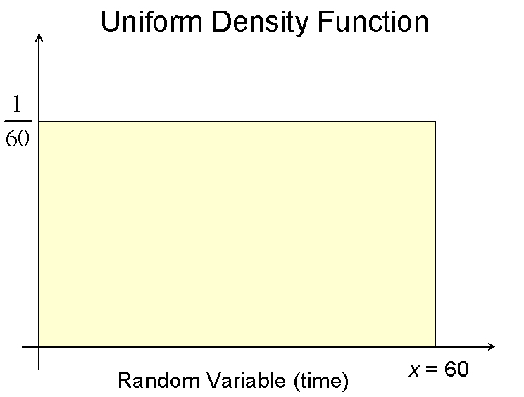
Because the area of a rectangle is length times width, and the width of the rectangle is 60, the height must be 1/60
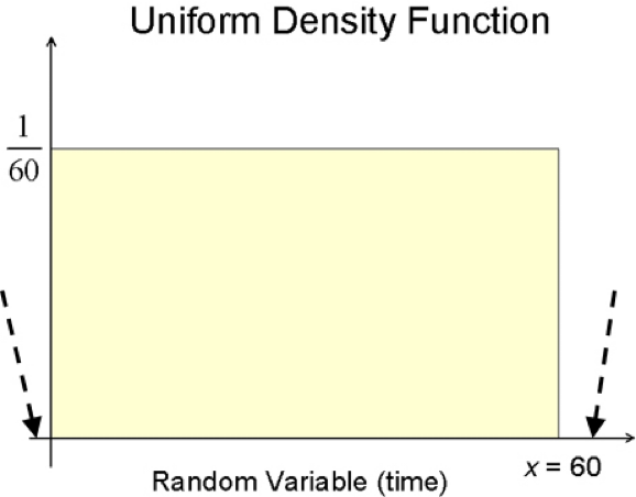
Values of the random variable X less than 0 or greater than 60 are impossible, thus the function value must be zero for X less than 0 or greater than 60.
The area under the graph of the density function over an interval represents the probability of observing a value of the random variable in that interval.
EXAMPLE Area as a Probability
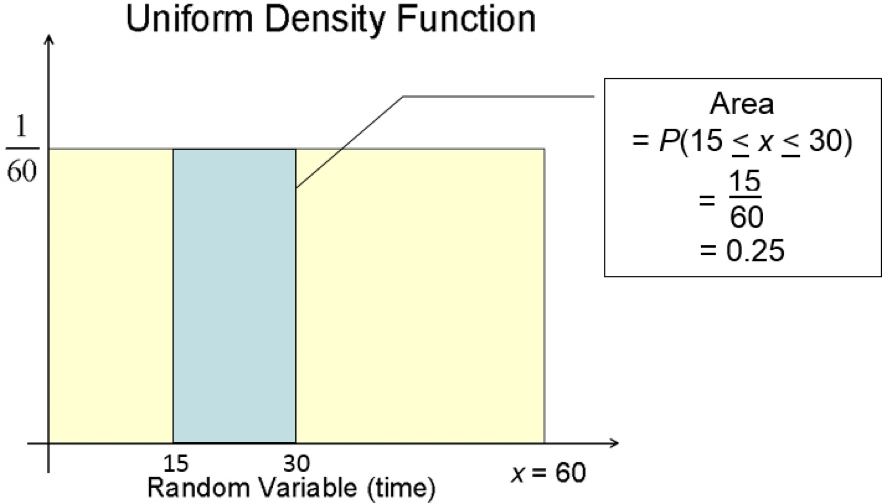
The probability of choosing a time that is between 15 and 30 minutes after the hour is the area under the uniform density function. “Probability that x is between 15 and 30 minutes” is what the equation below means.
Graphing a Normal Curve
Relative frequency histograms that are symmetric and bell-shaped are said to have the shape of a normal curve.
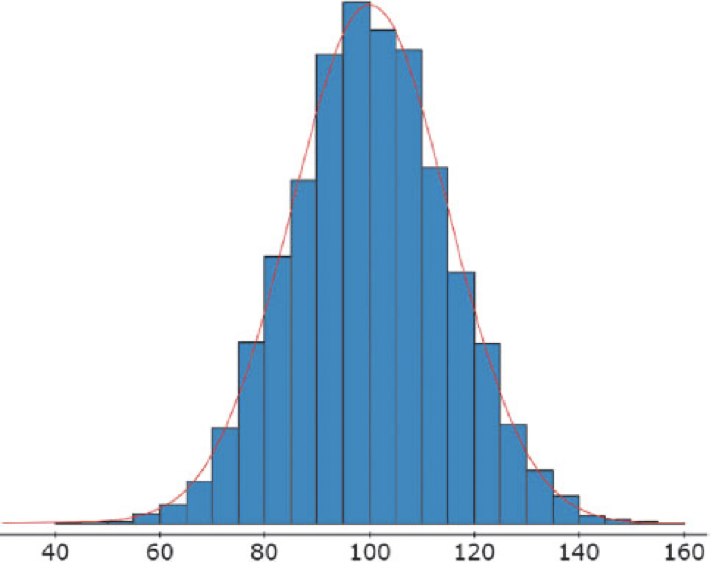
A normal distribution is a type of continuous probability distribution in which most data points cluster toward the middle of the range, while the rest taper off symmetrically toward either extreme. The middle of the range is also known as the mean of the distribution.
So, a continuous random variable is normally distributed, or has a normal probability distribution, if its relative frequency histogram of the random variable has the shape of a normal curve (bell-shaped and symmetric).
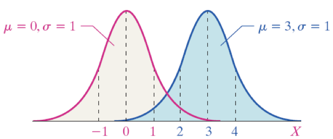
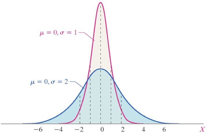
Difference between normal density function and normal random variable
A "normal density function" is the mathematical equation that describes the shape of a normal distribution, essentially a bell-shaped curve, while a "normal random variable" is a variable that is drawn from that normal distribution, meaning its possible values follow the pattern of the density function; in simpler terms, the density function is the formula that defines the probability of a normal random variable taking on a specific value within the distribution.
Properties of the Normal Density Curve
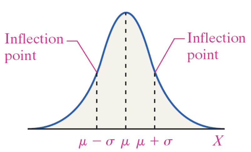
It is symmetric about its mean, μ.
Because mean = median = mode, the curve has a single peak and the highest point occurs at x = μ.
It has inflection points at μ + σ and μ − σ (who cares?!?!)
The area under the curve is 1.
The area under the curve to the right of μ = area under the curve to the left of μ, which is 1/2.
As x increases without bound (gets larger and larger), the graph approaches, but never reaches, the horizontal axis. As x decreases without bound (gets more and more negative), the graph approaches, but never reaches, the horizontal axis.
The Empirical Rule applies as well
ER: “Approximately 68% of the area under the normal curve is between x = μ − σ and x = μ + σ; approximately 95% of the area is between x = μ − 2σ and x = μ + 2σ; approximately 99.7% of the area is between x = μ − 3σ and x = μ + 3σ.”
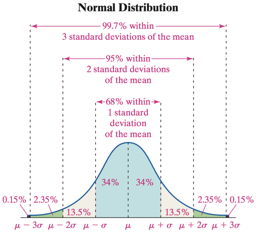
Area under a Normal Curve
When a random variable X is normally distributed with mean μ and standard deviation σ, the area under the normal curve for any interval of values of the random variable X represents either…
the proportion of the population with the characteristic described by the interval of values
or,
the probability that a randomly selected individual from the population will have the characteristic described by the interval of values.
EXAMPLE Normal Random Variable
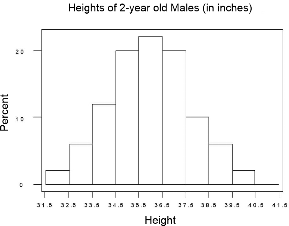
The data below represent the heights (in inches) of a random sample of 50 two-year old males.
36.0 | 36.2 | 34.8 | 36.0 | 34.6 | 38.4 | 35.4 | 36.8 |
34.7 | 33.4 | 37.4 | 38.2 | 31.5 | 37.7 | 36.9 | 34.0 |
34.4 | 35.7 | 37.9 | 39.3 | 34.0 | 36.9 | 35.1 | 37.0 |
33.2 | 36.1 | 35.2 | 35.6 | 33.0 | 36.8 | 33.5 | 35.0 |
35.1 | 35.2 | 34.4 | 36.7 | 36.0 | 36.0 | 35.7 | 35.7 |
38.3 | 33.6 | 39.8 | 37.0 | 37.2 | 34.8 | 35.7 | 38.9 |
37.2 | 39.3 |
(a) Draw a histogram of the data using a lower class limit of the first class equal to 31.5 and a class width of 1.
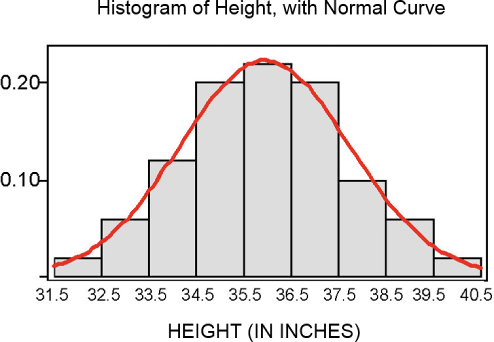
(b) Do you think that the variable “height of 2-year old males” is normally distributed?
Yes
EXAMPLE Explain the Role of Area in the Normal Density Function
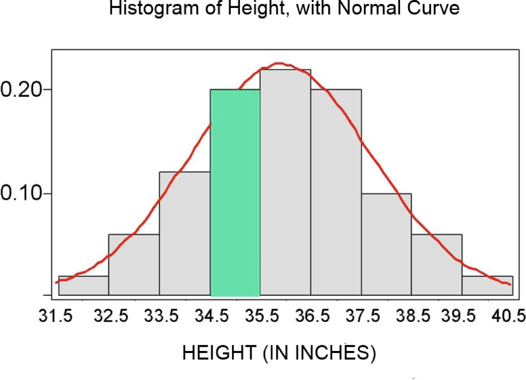
Here we have a normal density curve drawn over the histogram. How does the area of the rectangle corresponding to a height between 34.5 and 35.5 inches relate to the area under the curve between these two heights?
EXAMPLE Interpreting the Area Under a Normal Curve
The weights of giraffes are approximately normally distributed with mean μ = 2200 pounds and standard deviation σ = 200 pounds.
( a ) Draw a normal curve with the parameters labeled.
( b ) Shade the area under the normal curve to the left of x = 2100 pounds.
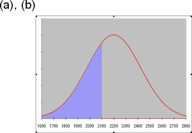
( c ) Suppose that the area under the normal curve to the left of x = 2100 pounds is 0.3085. Provide two interpretations of this result.
The proportion of giraffes whose weight is less than 2100 pounds is 0.3085
The probability that a randomly selected giraffe weighs less than 2100 pounds is 0.3085.
7.1 Properties of the Normal Distribution
Learning Objectives:
1. Use the uniform probability distribution
2. Graph a normal curve
3. State the properties of the normal curve
4. Explain the role of area in the normal density function
Probability density function (PDF) for a continuous random variable:
A Probability Density Function (PDF) is an equation used to compute probabilities of continuous random variables.
Generally applies to continuous random variables, where the function itself defines the probability density at each point in the variable’s range.
What is Density?
"density" in a PDF refers to the concentration of probability around each point
"density" in a PDF is not the probability itself.
By integrating density over an interval, we obtain the actual probability of the variable lying within that range.
What is Interval?
"interval" in a PDF refers to a specific range of values within which we want to calculate the probability for a continuous random variable.
In summary, a PDF is a function that, when integrated over an interval, provides the probability that a continuous random variable x falls within that interval. Rather than giving a probability for a single value, it describes the probability distribution across ranges, enabling us to calculate the likelihood of x within any specified interval. The area under the graph of the density function over an interval represents the probability of observing a value of the random variable in that interval.
A PDF must satisfy the following two properties:
The total area under the graph of the equation over all possible values of the random variable must equal 1.
The height of the graph of the equation must be greater than or equal to 0 for all possible values of the random variable.
What Is Uniform Distribution?
A random variable is said to follow a uniform probability distribution when…
Any two intervals of equal length are:
inclusive (between two stated variables)
equally likely
EXAMPLE ILLUSTRATING the Uniform Distribution
“ Suppose that United Parcel Service is supposed to deliver a package to your front door and the arrival time is somewhere between 10 am and 11 am. Let the random variable X represent the time from 10 am when the delivery is supposed to take place. The delivery could be at 10 am (x = 0) or at 11 am (x = 60) with all 1-minute interval of times between x = 0 and x = 60 equally likely. That is to say your package is just as likely to arrive between 10:15 and 10:16 as it is to arrive between 10:40 and 10:41. The random variable X can be any value in the interval from 0 to 60, that is, 0 < X < 60. Because any two intervals of equal length between 0 and 60, inclusive, are equally likely, the random variable X is said to follow a uniform probability distribution.”
The graph below illustrates the properties for the “time” example. Notice the area of the rectangle is one and the graph is greater than or equal to zero for all x between 0 and 60, inclusive.

Because the area of a rectangle is length times width, and the width of the rectangle is 60, the height must be 1/60

Values of the random variable X less than 0 or greater than 60 are impossible, thus the function value must be zero for X less than 0 or greater than 60.
The area under the graph of the density function over an interval represents the probability of observing a value of the random variable in that interval.
EXAMPLE Area as a Probability
The probability of choosing a time that is between 15 and 30 minutes after the hour is the area under the uniform density function. “Probability that x is between 15 and 30 minutes” is what the equation below means.

Graphing a Normal Curve
Relative frequency histograms that are symmetric and bell-shaped are said to have the shape of a normal curve.

A normal distribution is a type of continuous probability distribution in which most data points cluster toward the middle of the range, while the rest taper off symmetrically toward either extreme. The middle of the range is also known as the mean of the distribution.
So, a continuous random variable is normally distributed, or has a normal probability distribution, if its relative frequency histogram of the random variable has the shape of a normal curve (bell-shaped and symmetric).


Difference between normal density function and normal random variable
A "normal density function" is the mathematical equation that describes the shape of a normal distribution, essentially a bell-shaped curve, while a "normal random variable" is a variable that is drawn from that normal distribution, meaning its possible values follow the pattern of the density function; in simpler terms, the density function is the formula that defines the probability of a normal random variable taking on a specific value within the distribution.
Properties of the Normal Density Curve
It is symmetric about its mean, μ.
Because mean = median = mode, the curve has a single peak and the highest point occurs at x = μ.
It has inflection points at μ + σ and μ − σ (who cares?!?!)
The area under the curve is 1.
The area under the curve to the right of μ = area under the curve to the left of μ, which is 1/2.
As x increases without bound (gets larger and larger), the graph approaches, but never reaches, the horizontal axis. As x decreases without bound (gets more and more negative), the graph approaches, but never reaches, the horizontal axis.
The Empirical Rule applies as well
ER: “Approximately 68% of the area under the normal curve is between x = μ − σ and x = μ + σ; approximately 95% of the area is between x = μ − 2σ and x = μ + 2σ; approximately 99.7% of the area is between x = μ − 3σ and x = μ + 3σ.”

Area under a Normal Curve
When a random variable X is normally distributed with mean μ and standard deviation σ, the area under the normal curve for any interval of values of the random variable X represents either…
the proportion of the population with the characteristic described by the interval of values
or,
the probability that a randomly selected individual from the population will have the characteristic described by the interval of values.
EXAMPLE Normal Random Variable
The data below represent the heights (in inches) of a random sample of 50 two-year old males.
36.0 | 36.2 | 34.8 | 36.0 | 34.6 | 38.4 | 35.4 | 36.8 |
34.7 | 33.4 | 37.4 | 38.2 | 31.5 | 37.7 | 36.9 | 34.0 |
34.4 | 35.7 | 37.9 | 39.3 | 34.0 | 36.9 | 35.1 | 37.0 |
33.2 | 36.1 | 35.2 | 35.6 | 33.0 | 36.8 | 33.5 | 35.0 |
35.1 | 35.2 | 34.4 | 36.7 | 36.0 | 36.0 | 35.7 | 35.7 |
38.3 | 33.6 | 39.8 | 37.0 | 37.2 | 34.8 | 35.7 | 38.9 |
37.2 | 39.3 |
(a) Draw a histogram of the data using a lower class limit of the first class equal to 31.5 and a class width of 1.
(b) Do you think that the variable “height of 2-year old males” is normally distributed?
Yes
EXAMPLE Explain the Role of Area in the Normal Density Function
Here we have a normal density curve drawn over the histogram. How does the area of the rectangle corresponding to a height between 34.5 and 35.5 inches relate to the area under the curve between these two heights?


EXAMPLE Interpreting the Area Under a Normal Curve
The weights of giraffes are approximately normally distributed with mean μ = 2200 pounds and standard deviation σ = 200 pounds.
( a ) Draw a normal curve with the parameters labeled.
( b ) Shade the area under the normal curve to the left of x = 2100 pounds.

( c ) Suppose that the area under the normal curve to the left of x = 2100 pounds is 0.3085. Provide two interpretations of this result.
The proportion of giraffes whose weight is less than 2100 pounds is 0.3085
The probability that a randomly selected giraffe weighs less than 2100 pounds is 0.3085.
