IER Notes 1 , 13-16
IER Notes
Chapter 1 : trade in the global economy
- international trade
Baiscs of world trade
Export : selling products from one country to another
Import : buying products from another country
- Trade Balance:the difference between the total value of its exports and imports. If a country exports more than it imports, it has a trade surplus, and if it imports more than it exports, it has a trade deficit.
- Bilateral Trade Balance: This refers to the trade balance between two specific countries. For example, the trade balance between the United States and China.
- Assumption of Balanced Trade: In economic models, it's assumed that each country has balanced trade, with exports equaling imports. This assumption simplifies analysis.
- Macroeconomic Factors: Trade deficits or surpluses are influenced by factors like overall spending and savings within an economy.
- Complexity of Trade: The value of products can involve components from multiple countries. For instance, even though an iPhone may be assembled in China, many of its parts are imported from other countries. This complexity challenges the accuracy of bilateral trade balances.
- Offshoring: Modern trade involves manufacturing processes spread across multiple countries, known as offshoring. This trend has increased due to reduced transportation and communication costs.
- World Trade Map: The map in Figure 1-2 illustrates the flow of exports and imports around the world in 2014, with trade in goods totaling about $19.8 trillion. Services are not included in the map due to measurement complexities.
- Trade in Goods vs. Services:
- Goods: These are physical products traded between countries. The map visualizes the flow of goods based on the width of the lines, with thicker lines representing larger trade volumes.
- Services: While not depicted in the map, services like tourism, financial services, and entertainment also contribute to international trade, though they are more challenging to measure.
- Regional Trade Highlights:
- Europe: Trade within Europe is substantial, accounting for almost one-quarter of world trade in 2014. The European Union (EU) fosters trade among its 28 member countries by imposing zero tariffs on imports from one another.
- Americas: Trade within the Americas, including North, Central, and South America, and the Caribbean, is significant, totaling about 9% of world trade.
- Asia: Asia accounts for about one-third of world trade, with China being a major exporter to the United States and other regions.
- Middle East and Russia: These regions, known for their oil reserves, also contribute significantly to global trade.
- Trade Barriers and Changes Over Time:
- Tariffs: Historical data show fluctuations in tariffs, with a notable increase during the interwar period due to policies like the Smoot-Hawley Tariff Act. High tariffs can reduce trade and impose costs on economies.
- Global Financial Crisis: The financial crisis of 2008-2009 led to a slowdown in international trade, affecting many countries.
- Future of Trade:
- Free Trade Areas: Negotiations for free trade agreements like the Trans-Pacific Partnership and the Transatlantic Trade and Investment Partnership aim to reduce tariffs and promote trade.
- Climate Change: Global warming may impact trade patterns, with the melting Arctic ice opening new shipping routes and opportunities for trade
1.2. Migration & foreging direct investement
Migration: the movement of people across borders,
foreign direct investment: the movement of capital across borders.
This part is on global migration patterns & the movement of people from low-wage to high-wage countries and the policies surrounding immigration in the European Union (EU) and the United States.
- Global Migration Trends:
- More than half (60%) of the 232 million foreign-born people worldwide come from countries outside the Organisation for Economic Co-operation and Development (OECD).
- Asia has the highest number of migrants (68 million), followed by Africa (19 million) and Latin America (9 million).
- Restrictions on Immigration:
- Policy makers in OECD countries often implement restrictions on immigration, fearing that immigrants from low-wage countries will lower wages for local workers.
- Immigration policies are a hotly debated political issue in many countries, including Europe and the United States.
- Role of International Trade:
- International trade can act as a substitute for labor movement, raising living standards for workers in exporting industries.
- Increased openness to trade since World War II has provided opportunities for workers to benefit through trade, even when migration restrictions prevent them from directly earning higher incomes abroad.
- European Union Immigration Policies:
- Labor mobility was very open within the EU prior to 2004.
- Expansion of the EU to include central European countries led to concerns about labor migration from low-wage to high-wage countries.
- The Schengen Area allows for open borders between EU countries, except for the UK and Ireland.
- United States Immigration Policies:
- The United States has a significant population of Latin American immigrants, particularly from Mexico.
- Immigration policy is a frequent topic of debate, especially during presidential elections.
- Various attempts at immigration reform have been made, but comprehensive reform has not been achieved.
- 2016 US Presidential Election:
- During the 2016 election campaign, immigration was a prominent issue.
- Donald Trump proposed expelling all illegal Mexican immigrants and building a wall between the US and Mexico.
- Other Republican candidates also took strong stands against illegal immigration.
foreign direct investment (FDI) occurs when a firm in one country owns (in part or in whole) a company or property in another country.
- FDI can be described in one of two ways: as horizontal FDI or vertical FDI.
Horizental FDI
Horizontal FDI refers to the investment made by a company from one industrialized country into a company located in another industrialized country. This type of investment typically involves the acquisition of a company rather than the establishment of new facilities. The passage provides examples of horizontal FDI, such as the purchase of Tim Hortons by Burger King in 2014.
There are several reasons why companies engage in horizontal FDI:
- Tax Avoidance: One major reason is to minimize taxes. By moving headquarters to a country with lower corporate income tax rates or by strategically locating subsidiaries in countries with favorable tax policies, companies can reduce their tax burden.
- Market Access: Establishing a presence in another country provides improved access to that market. Local subsidiaries have better knowledge of the market and can facilitate marketing and distribution of products more effectively.
- Competitive Advantage: Horizontal FDI allows companies to leverage the strengths of both the acquiring and acquired firms. For example, combining expertise in different product lines or market segments can strengthen the competitiveness of the combined entity against competitors.
- Resource Sharing: Collaboration between production divisions of different firms allows for the sharing of technical expertise and resources, reducing duplication of efforts and costs. This can lead to greater efficiency and innovation.
Overall, horizontal FDI enables firms to expand their business operations across borders by acquiring existing companies in other industrialized countries.
Top of Form
Vertical FDI
Vertical FDI occurs when a company from an industrialized country owns a plant or facility in a developing country. Unlike horizontal FDI, which involves investment between industrialized countries, vertical FDI typically involves outsourcing production to take advantage of lower labor costs in developing countries.
The primary motivation behind vertical FDI is the pursuit of cost savings, particularly in labor expenses. Companies from industrialized economies seek to leverage their technological expertise and combine it with the cheaper labor available in developing countries. This allows them to produce goods more cost-effectively for the global market.
- China serves as a prominent example of vertical FDI, where many companies have established manufacturing facilities to capitalize on the country's abundant labor force and lower production costs. These firms often partner with local entities to navigate regulatory hurdles and gain access to the Chinese market.
In addition to cost savings, companies may also use vertical FDI to avoid tariffs and gain easier access to local markets. For instance, foreign automobile manufacturers have set up production plants in China, often in partnership with local companies, to circumvent high import tariffs and better serve the domestic market.
Despite China's reduction in tariffs following its accession to the World Trade Organization in 2001, foreign firms continue to maintain their manufacturing presence in the country. In fact, some are now exploring opportunities to export products manufactured in China to other markets.
Vertical FDI represents a strategy employed by multinational corporations to optimize their production processes, lower costs, and enhance their competitiveness in the global marketplace.
Largest stocks of FDI are in Europe ,
CCL
Globalization encompasses many aspects, like the flow of goods, services, people, and firms across borders, as well as the spread of culture and ideas globally. While it may seem like a modern phenomenon, globalization has historical roots, with strong international trade and financial integration existing before World War I. However, global linkages were disrupted by the war and the Great Depression. Since World War II, there has been a rapid resurgence of global trade, outpacing the growth in world GDP, facilitated by international institutions like the World Trade Organization, the International Monetary Fund, and others established to promote freer trade and economic development.
Migration across countries, unlike international trade, faces restrictions due to concerns about its impact on wages. However, these fears may not always be justified, as immigrants can often be assimilated into host countries without adversely affecting wages. Foreign Direct Investment (FDI), on the other hand, is relatively unrestricted in industrialized countries but may face limitations in developing countries. Firms invest in different countries to capitalize on factors like lower wages and to spread their business operations and production knowledge across borders. Migration and FDI are integral components of contemporary globalization.
Key points to consider:
- The trade balance of a country depends on macroeconomic conditions and is determined by the difference between its exports and imports.
- The nature of traded goods has evolved from raw materials and basic processed goods to highly processed consumer and capital goods, with goods often crossing borders multiple times during manufacturing.
- A significant portion of international trade occurs between industrialized countries, with Europe and the United States accounting for a substantial share.
- Trade models often emphasize differences between countries, but trade between similar countries also occurs, involving the exchange of different varieties of goods.
- Larger countries tend to have smaller trade-to-GDP ratios due to significant internal trade. However, smaller economies like Hong Kong and Singapore have high trade-to-GDP ratios.
- Most world migration originates from developing countries, with migrants often seeking entry into wealthier, industrialized countries.
- International trade serves as a substitute for migration, allowing workers to improve their standard of living by working in export industries, even if they cannot migrate.
- The majority of world FDI occurs between industrialized countries, with Europe and the United States being significant participants. The OECD countries account for a substantial share of global FDI flows.
The debate over whether the European Central Bank (ECB) should raise interest rates to counter inflation is a complex one, with arguments on both sides.
Arguments for Raising Interest Rates:
- Taming Inflation: Higher interest rates can be used as a tool to curb inflation by reducing the amount of money circulating in the economy. When interest rates rise, borrowing becomes more expensive, leading to reduced spending and investment, which can help slow down inflationary pressures.
- Maintaining Price Stability: Central banks like the ECB have a mandate to maintain price stability, which often means keeping inflation within a target range. Raising interest rates can be seen as a proactive measure to ensure that inflation doesn't spiral out of control, which could have detrimental effects on consumers' purchasing power and overall economic stability.
- Preserving Credibility: Central banks' credibility is closely tied to their ability to control inflation. If inflation persists above target levels for too long without a response from the central bank, it could undermine public confidence in the bank's ability to fulfill its mandate, potentially leading to higher inflation expectations and further exacerbating the problem.
Arguments against Raising Interest Rates:
- Risk to Economic Recovery: Raising interest rates could potentially slow down economic growth, particularly if it's done too quickly or aggressively. Higher borrowing costs can discourage investment and consumption, which are crucial drivers of economic activity. In an environment where many European countries are still recovering from the economic impacts of the COVID-19 pandemic, overly restrictive monetary policy could derail progress.
- Debt Servicing Costs: Higher interest rates would increase the cost of servicing government and private sector debt. European countries, particularly those with high levels of public debt, could face significant challenges in managing their debt burdens if interest rates rise, potentially leading to fiscal strains and even sovereign debt crises in extreme cases.
- Exchange Rate Implications: Raising interest rates could lead to an appreciation of the euro against other currencies, which could negatively impact European exporters by making their goods more expensive in foreign markets. This could further dampen economic activity and exacerbate any slowdown resulting from higher interest rates.
In conclusion, the decision to raise interest rates to counter inflation involves weighing the immediate need to control price pressures against the potential risks to economic growth, debt sustainability, and exchange rate dynamics. The ECB must carefully assess the current economic conditions and inflation outlook to determine the appropriate course of action that balances these competing concerns.
COVID-19 Pandemic:
During the COVID-19 pandemic, central banks around the world, including the ECB, implemented aggressive monetary policy measures to support economies reeling from lockdowns and disruptions. Interest rates were slashed to historically low levels to stimulate borrowing and spending and to prevent a deeper economic downturn.
Impact on Popular Companies:
- Airline Industry: Companies like Lufthansa, British Airways, and Air France-KLM faced significant challenges due to travel restrictions and reduced demand for air travel. Low interest rates helped these companies access cheaper financing to weather the crisis, but the sector's recovery was heavily dependent on factors like vaccine distribution and easing travel restrictions.
- Hospitality and Tourism: Hotel chains like Marriott International and Hilton Worldwide experienced a sharp decline in bookings as travel ground to a halt. Low interest rates provided some relief by reducing borrowing costs for expansion or renovation projects, but the industry's recovery was slow and uneven as consumer confidence remained subdued.
- Retail Sector: Retail giants like H&M, Inditex (owner of Zara), and Macy's faced store closures and reduced foot traffic during lockdowns. Low interest rates supported consumer spending by reducing the cost of credit card debt and mortgages, but brick-and-mortar retailers struggled to adapt to changing consumer preferences and the rise of e-commerce.
Great Recession:
During the Great Recession of 2008-2009, central banks responded to the financial crisis by lowering interest rates and implementing unconventional monetary policy measures like quantitative easing to stabilize financial markets and stimulate economic growth.
Impact on Popular Companies:
- Automotive Industry: Companies like General Motors and Ford faced a sharp decline in demand for cars and trucks as consumer spending contracted and credit markets froze. Low interest rates helped support auto sales by reducing the cost of financing for car loans, but the industry faced restructuring and consolidation as weaker players struggled to survive.
- Financial Institutions: Banks like Lehman Brothers and Bear Stearns collapsed during the financial crisis due to exposure to toxic assets and liquidity problems. Low interest rates and government interventions like bailouts and liquidity injections helped stabilize the financial system and restore confidence, but regulatory reforms were implemented to prevent future crises.
- Technology Sector: Companies like Apple and Google weathered the Great Recession better than many traditional industries due to their strong balance sheets and innovative products. Low interest rates and government stimulus measures indirectly supported tech spending by boosting consumer and business confidence, but the sector still faced challenges like reduced corporate IT budgets and weaker demand for high-end gadgets.
In both the COVID-19 pandemic and the Great Recession, low interest rates played a critical role in supporting economic recovery and mitigating the impact of the crises on popular companies. However, the debate around raising interest rates to counter inflation remains relevant as economies gradually recover and central banks seek to prevent overheating and financial imbalances.
Bottom of FormChapter 12 : the global macroeconomy
1. Why do exchange rates matter and what explains their behavior?
2. Why do countries borrow from and lend to eachother and with what effects?
3. How do government policy choices affect macroeconomic outcomes?
12.1 Foreign exchange : currencies & crises
Exchange rates : the value of one currency in terms of another currency. They determine the price at which one currency can be exchanged for another in the foreign exchange market.
- Exchange rates are crucial for international trade and investment because they influence the cost of goods and services between countries, as well as the profitability of cross-border transactions.
The main purpose of exchange rates is to facilitate international trade and investment by providing a way to convert one currency into another. They help businesses and individuals assess the relative value of different currencies and make decisions about imports, exports, and investments. Exchange rates also influence a country's economic stability, impacting its balance of trade, inflation rate, and overall competitiveness. Governments and central banks often intervene in currency markets to manage exchange rates and achieve economic goals, such as controlling inflation or promoting exports.
How Exchange rates behave
Exchange rates behave differently depending on the monetary policies of the countries involved.
Either they’re Fixed/ pegged or Stable Exchange Rates, like the Chinese yuan in relation to the US dollar, have relatively stable exchange rates, which are often fixed or pegged to another currency.
- This means their value remains consistent over time, with minor fluctuations controlled by the government. In a fixed exchange rate system, the government or central bank sets the value of the currency relative to another currency, maintaining stability but limiting flexibility
Currencies can also be Floating or Flexible Exchange Rates like the euro in relation to the US dollar have floating exchange rates, which fluctuate more widely based on market forces like supply and demand.
In contrast, a floating exchange rate system allows the currency's value to be determined by market forces, resulting in more frequent and larger fluctuations in the exchange rate.
Several market factors contribute to the flexibility of exchange rates:
- Supply and Demand for Currencies: Like any other market, the foreign exchange market operates based on the forces of supply and demand. If there's high demand for a particular currency, its value relative to other currencies will increase, and vice versa. Factors affecting demand include trade balances, investment flows, and geopolitical events.
- Interest Rates: Central banks' monetary policy decisions, particularly regarding interest rates, play a crucial role in exchange rate movements. Higher interest rates attract foreign investment, leading to increased demand for a currency and thus appreciation. Conversely, lower interest rates may lead to depreciation as investors seek higher returns elsewhere.
- Inflation Rates: Countries with lower inflation rates generally see an appreciation of their currency because their purchasing power increases. Conversely, higher inflation rates can lead to currency depreciation as the cost of goods and services rises relative to other currencies.
- Economic Performance: Exchange rates are influenced by a country's economic performance indicators such as GDP growth, unemployment rates, and industrial production. Strong economic performance attracts foreign investment, driving up demand for the currency and its value.
- Political Stability and Economic Policies: Countries with stable political environments and sound economic policies tend to have more stable currencies. Political instability, corruption, or unpredictable economic policies can lead to currency depreciation as investors lose confidence in the currency's value.
- Speculation: Traders and investors in the foreign exchange market engage in speculative activities based on their expectations of future exchange rate movements. Speculation can lead to short-term fluctuations in exchange rates, especially in response to news events or market sentiment.
Why exchange rates matter
Exchange rates matter for several reasons:
- Impact on International Trade: Changes in exchange rates affect the relative prices of goods and services between countries. When a currency appreciates (increases in value), exports become more expensive for foreign buyers, potentially reducing demand for those goods and leading to a decline in exports. Conversely, a depreciating currency makes exports cheaper and can stimulate foreign demand. This can have significant implications for businesses that rely on international trade, as illustrated by the Swiss cheesemaker's dilemma in the example.
- Effect on Asset Prices: Exchange rate fluctuations also influence the relative value of assets held in different currencies. For example, when the value of a currency falls, the value of assets denominated in that currency decreases when converted into another currency. This can lead to capital gains or losses for investors holding foreign assets, impacting their wealth and investment decisionS.
- International Investment: Exchange rate movements affect the attractiveness of investing in foreign markets. A stronger domestic currency makes foreign investments cheaper for domestic investors, while a weaker currency makes domestic assets more attractive to foreign investors. This can influence capital flows across borders and impact investment decisions made by firms, governments, and individuals.
- Economic Stability: Exchange rate stability is crucial for maintaining economic stability and confidence in the financial system. Sharp fluctuations in exchange rates can disrupt trade, investment, and financial markets, leading to uncertainty and volatility. Central banks often intervene in currency markets to stabilize exchange rates and support economic stability.
- International Trade: They determine the prices of goods sold between countries. When a currency goes up, exports become more expensive, and when it goes down, exports become cheaper.
- Asset Prices: Changes in exchange rates can affect the value of investments held in different currencies. This can lead to gains or losses for investors.
- International Investment: Exchange rates influence the attractiveness of investing in foreign markets. A strong domestic currency makes foreign investments cheaper, while a weak currency makes domestic assets more appealing.
- Economic Stability: Stable exchange rates are important for keeping the economy steady. Big changes can cause uncertainty and disrupt trade and investments. Central banks sometimes step in to keep exchange rates stable.
When exchanges misbehave
Exchange rate crises occur when a currency suddenly loses value against another currency after a period of stability. These crises can lead to severe economic and social consequences, as seen in Argentina's crisis in 2001-2002. During this time, the Argentine peso, which had been fixed to the U.S. dollar, lost value rapidly, leading to financial chaos, debt default, high inflation, unemployment, and widespread poverty.
Argentina's experience is not unique, as exchange rate crises have occurred in many countries. From 1997 to 2015, there were 32 such crises, often resulting in significant economic downturns and political instability. Countries affected include those in East Asia, as well as Liberia, Russia, Brazil, Iceland, and Ukraine.
During exchange rate crises, output decreases, banking and debt problems emerge, and political turmoil often follows. Governments may seek external help from organizations like the International Monetary Fund (IMF) or the World Bank to address the crisis. These events highlight the importance of understanding and addressing exchange rate dynamics, especially during times of crisis.
Top of Form
12.2 Globalization of finance : debts & deficits
Deficits & surplus : the balance of payments
The balance of payments : to the tracking of a country's economic transactions with the rest of the world.
The balance of payments, much like personal finances, involves tracking income and expenditure. If income exceeds expenditure, there's a surplus, but if expenditure surpasses income, there's a deficit. This difference between income & expenditure is known as the current account, indicates whether a country is living within its means.
- If a country's income exceeds its expenditure, it has a current account surplus, indicating that it is exporting more than it imports and is a net lender to the rest of the world. Conversely, if expenditure exceeds income, the country has a current account deficit, suggesting that it is borrowing from the rest of the world to finance its excess spending.
For instance, in the United States, expenditure has often exceeded income since 1990, resulting in a current account deficit, except for a small surplus in 1991. To cover this deficit, the U.S. borrows from the rest of the world through financial transactions, similar to how households might manage deficits by borrowing money.
Since the world economy operates as a closed system, with no external borrowing sources, if one country like the U.S. runs a deficit, others must run surpluses. Thus, while individual countries may have deficits or surpluses, globally, the finances balance out.
Understanding the balance of payments is crucial for assessing a country's economic health and its position in the global economy. It reflects whether a country is living within its means or relying on external borrowing to sustain its economic activities.
Debtors & creditors : External wealthBottom of Form
Wealth/net worth : Assets ( what others owe you) – liabilities (what u owe).
External wealth is a country's net worth and it’s the difference between its foreign assets (what it is owed by the rest of the world) and its foreign liabilities (what it owes to the rest of the world).
- Creditor Nation: When a country's external wealth is positive, it means that other nations owe it money. In other words, it's a creditor nation.
- Debtor Nation: Conversely, if a country's external wealth is negative, it indicates that it owes money to other nations, making it a debtor nation.
Changes in a nation's external wealth are influenced by its current account balance. A surplus leads to an increase in external wealth, while a deficit causes it to decline.
Ex: persistent current account deficits in the United States since the 1980s have contributed to a significant decrease in its external wealth, making it the world's largest debtor by the second quarter of 2015. Similarly, Argentina's external wealth declined due to its recurring current account deficits in the 1990s.
However, external wealth isn't solely determined by income and expenditure. Factors like capital gains or losses on investments, as well as deliberate actions such as debt defaults, also play a role. For example, Argentina's external wealth increased in 2002 despite defaulting on its government debt, as it simultaneously reduced its liabilities. Therefore, fluctuations in external wealth can occur not only due to economic imbalances but also due to market dynamics and policy decisions.
Darling & deadbeats : defaults and other risks
Defaults on government debt are not uncommon in international finance. Since 1980, several countries have defaulted on private creditors multiple times, including Argentina, Chile, Ecuador, Greece, Indonesia, Mexico, Nigeria, and others. Additionally, countries that fail to make payments on loans from international financial institutions, like the World Bank, could also be considered in default, although such cases may be managed to avoid formal default.
Sovereign governments typically have the power to default on their debt without facing legal consequences. They can also impact creditors through various means, such as seizing assets or changing laws and regulations after investments have been made.
To mitigate these risks, international investors carefully assess and monitor debtors. Nations and firms are assigned credit ratings based on their financial behavior. A high credit rating indicates low risk and provides access to low-interest loans, while a low rating means higher interest rates and limited credit.
Countries issuing bonds to raise funds are also rated by agencies like Standard & Poor's (S&P). Bonds rated BBB- or higher are considered investment-grade, while those rated BB+ and lower are classified as junk bonds. Poorer ratings are associated with higher interest rates, with the difference between rates on safe U.S. Treasury bonds and bonds from riskier countries termed as country risk. For instance, on January 8, 2016, Poland and Mexico had relatively low country risk, while Brazil and Turkey faced higher penalties due to their lower credit ratings.
12.3. Gov & institutions : Policies & performance
Integration & Capital Controls : The regulation of International Finance
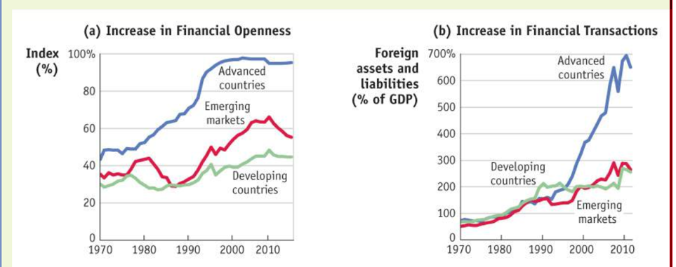 The trend towards financial globalization since 1970 is evident in Figure 12-5. Panel (a) displays an index of financial openness, which means it shows how open countries are to financial transactions. It's like a scale: 0% means countries have tight controls, while 100% means they're fully open. The graph divides countries into three groups: advanced, emerging, and developing.
Advanced countries, characterized by high levels of income per person and strong integration into the global economy, led the shift towards financial openness. In the 1980s, many of these countries abolished capital controls that had been in place since World War II. Emerging markets, middle-income countries experiencing growth and greater integration, also began opening up financially in the 1990s, albeit to a lesser extent. Developing countries, with lower income levels and less integration, followed suit, albeit slowly.
Panel (b) illustrates the consequence of these policy changes: a significant increase in cross-border financial transactions. Total foreign assets and liabilities, expressed as a fraction of output, surged by a factor of 10 or more as the world became more financially open. This trend was most pronounced in advanced countries but also evident in emerging markets and developing countries.
As an example of evading control, Zimbabwe implemented capital controls, requiring U.S. dollars to be traded for Zimbabwe dollars only through official channels at an official rate. However, unofficial street markets emerged, reflecting a different reality.
- Financial Openness: This refers to the degree to which a country's financial system allows for cross-border financial transactions, such as investment flows and capital movements. A fully financially open economy would have no restrictions on such transactions, while a closed economy would tightly control them.
- Capital Controls: These are rules set by governments to manage the flow of money entering and leaving their economies. Capital controls can take different forms, like limits on currency exchange, restrictions on foreign investments, or taxes on money moving across borders.
- Credit Ratings: These are evaluations of how likely a borrower, like a government or a company, is to repay its debts. Credit rating agencies provide these assessments to help investors gauge the risk of investing in the borrower's debt. Higher ratings mean lower risk, while lower ratings indicate higher risk.
- Country Risk: This is the extra risk investors face when investing in assets or securities from a specific country, compared to investing in something considered risk-free, like U.S. Treasury bonds. Country risk factors in things like political stability, economic performance, and the likelihood of a government defaulting on its debts. Higher country risk usually leads to higher interest rates for bonds issued by that country.
Independence & monetary policy : the choice of exchange rates regimes
Exchange rate regimes basically refer to how a country manages its currency in relation to other currencies. There are two main types: fixed and floating.
- Fixed regimes : involve setting a specific value for the exchange rate,
- floating regimes : allow the rate to be determined by market forces. Both types are common globally.
- Fixed Regimes: Under this system, a country sets a specific value for its currency against another currency or a basket of currencies. This value is usually maintained by the country's central bank through buying or selling its currency in the foreign exchange market. Many countries use fixed regimes to provide stability to their currency's value.
- Floating Regimes: In contrast, floating regimes allow a country's currency value to be determined by market forces like supply and demand. The exchange rate fluctuates freely based on factors like interest rates, economic indicators, and investor sentiment. This system gives countries more flexibility but can lead to volatile currency movements.
The choice of which regime to adopt is a big decision for policymakers and can have significant impacts on the economy. Some argue that fixed regimes offer stability but limit a country's ability to respond to economic changes, while floating regimes provide flexibility but can result in unpredictable currency values.
Despite the existence of many currencies globally, some regions have moved towards currency integration, like the Eurozone, where multiple countries share a common currency (the euro) and monetary policy responsibilities. Others have opted for using foreign currencies, relinquishing control over their monetary policy.
Governance
Institutions, often referred to as governance, encompass a range of factors such as legal, political, social, and cultural structures within a society. These elements play a crucial role in shaping a nation's economic prosperity and stability.
- Institutional Quality: It's measured using indicators like voice and accountability, political stability, government effectiveness, regulatory quality, rule of law, and control of corruption. Better-quality institutions are associated with higher levels of income per capita and lower income volatility.
- Exchange Rate Regimes: These are frameworks that dictate how a country manages its currency in relation to others. The two main types are fixed regimes, where the value is set against another currency, and floating regimes, where the value is determined by market forces.
- The Spence Report: This landmark report led by Michael Spence focuses on strategies for sustained growth and inclusive development. It highlights a shift away from universal policy prescriptions towards pragmatic, context-specific approaches. It emphasizes the importance of diagnosing specific economic bottlenecks and experimenting with targeted policy initiatives.
- Factors Influencing Institutional Variation: These include historical legacies like colonization, legal systems, and resource endowments. For example, regions settled by Europeans often developed better institutions compared to those without European influence.
Chapter 13 : Introduction to exchange rates & the foreign exchange market
13.1 exchange rate essentials
Exchange Rate: the price of one currency in terms of another currency. It tells you how much of one currency you need to buy a unit of another currency.
- Quoting Exchange Rates: Exchange rates can be quoted in two ways:
- Home Currency Units per Foreign Currency: This tells you how many units of your home currency you need to buy one unit of foreign currency.
- Foreign Currency Units per Home Currency: This tells you how many units of foreign currency you can buy with one unit of your home currency.
Example: If the exchange rate between the U.S. dollar and the euro is $1.15 per euro, it means you need $1.15 to buy one euro. Alternatively, you can express it as €0.87 per U.S. dollar, indicating you can buy €0.87 with one U.S. dollar.
Defining the exchange rates
When we talk about exchange rates, we're discussing the value of one currency compared to another. Typically, we express/ quote this as units of our home currency per unit of the foreign currency.
EX: if you're in the U.S., you might see the price of euros quoted as $1.15 per euro. But if you're in the Eurozone, you'd see it as €0.87 per U.S. dollar.
To keep things clear, we'll stick to one way of quoting exchange rates throughout this book: units of the home currency per unit of the foreign currency.
EX: if we're talking about the exchange rate between the U.S. dollar and the euro, we'll write it as E$/€ = 1.086, meaning $1.086 per euro from the U.S. perspective. Conversely, from the Eurozone perspective, it would be E€/$ = 0.921, indicating €0.921 per U.S. dollar.
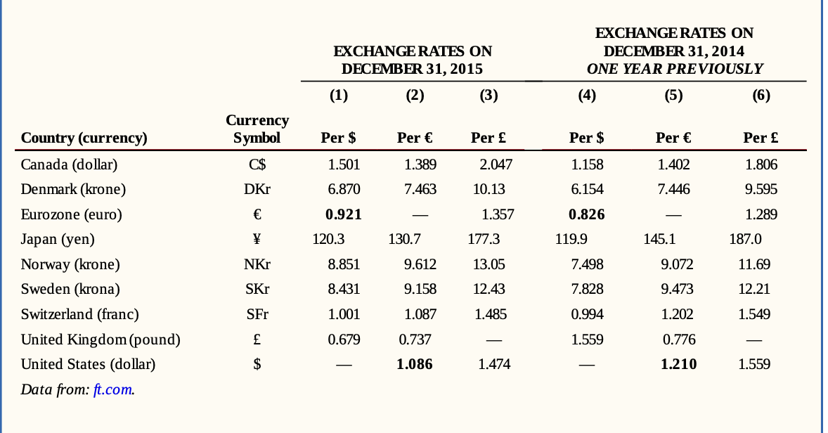 Remember, the value of one currency in terms of another always equals the reciprocal of the value of the second currency in terms of the first. So, E$/€ = 1/E€/$. In our example, 1.086 = 1/0.921.
Appreciations & Deprecoations
When we talk about exchange rates changing over time, we often use terms like appreciation and depreciation.
Appreciation : means that a currency has gained value compared to another currency
Depreciation : means it has lost value.
- Let's say the exchange rate between the U.S. dollar and the euro changes. If the exchange rate rises, it means more dollars are needed to buy one euro. This is called depreciation of the dollar because it's getting weaker compared to the euro. Conversely, if the exchange rate falls, fewer dollars are needed to buy one euro, indicating appreciation of the dollar against the euro.
The same applies from the Eurozone perspective. If the Eurozone exchange rate rises, it means more euros are needed to buy one dollar, indicating depreciation of the euro. If it falls, fewer euros are needed to buy one dollar, indicating appreciation of the euro against the dollar.
Interestingly, changes in exchange rates are always opposite for the two currencies involved. For example, if the dollar appreciates against the euro, it means the euro must depreciate against the dollar. This is because the two exchange rates are reciprocal of each other.
To measure how much a currency has appreciated or depreciated, we calculate the percentage change in its value relative to the other currency.
To calculate the percentage change:
- Find the difference between the new and old exchange rates.
- Divide the difference by the old exchange rate.
- Multiply by 100 to get the percentage change.
Example:
- Suppose the exchange rate for the U.S. dollar against the euro was $1.210 last year and $1.086 this year.
- The change is $1.086 - $1.210 = -$0.124.
- To find the percentage change: (-$0.124 / $1.210) * 100 = -10.25%.
- So, the euro depreciated against the dollar by 10.25%.
- Similarly, if the euro value of the dollar was €0.826 last year and €0.921 this year:
- The change is €0.921 - €0.826 = +€0.095.
- The percentage change is (+€0.095 / €0.826) * 100 = +11.50%.
- Therefore, the dollar appreciated against the euro by 11.50%.
- Note that the size of one country’s appreciation (here 11.50%) does not exactly equal the size of the other country’s depreciation (here 10.25%). For small changes, however, the opposing movements are approximately equal.
Multilatéral exchange rates
Multilateral exchange : Measure changes in a currency's value against many currencies.
- Accounts for trade weights to calculate an average of bilateral changes.
Calculation: To calculate the change in the effective exchange rate, economists use trade weights to aggregate bilateral exchange rate changes.
- Multiply each exchange rate change by its corresponding trade share.
- Add up the weighted changes to find the effective exchange rate change.
EX: If a country's currency appreciates 10% against 1 and depreciates 30% against 2, suppose 40% of Home trade is with country 1 and 60% is with country 2
- Multiply each change by the trade share and then add them up
- (−10% · 40%) + (30% · 60%) = (−0.1 · 0.4) + (0.3 · 0.6) = −0.04 + 0.18 = 0.14 = +14%.
Significance: Multilateral exchange rates provide a broader view of a currency's performance in the global market, considering its value relative to multiple currencies rather than just one.
Figure 13-1: The figure shows the change in the value of the U.S. dollar measured against two different baskets of foreign currencies. It illustrates how the dollar's value can vary depending on the currencies included in the basket and their respective trade relationships with the U.S.
Example: Using Exchange Rates to Compare Prices in a Common Currency
Top of Form
In this example, James Bond needs to compare tuxedo prices in different cities, each priced in its local currency: £2,000 in London, HK$30,000 in Hong Kong, and $4,000 in New York. To make a fair comparison, he converts all prices to a common currency using exchange rates.
- In Scenario 1, the Hong Kong tuxedo costs HK$30,000, divided by the exchange rate of HK$15 per £, equals £2,000. Similarly, the New York tuxedo priced at $4,000, divided by the exchange rate of $2 per £, also equals £2,000. Thus, both tuxedos are priced equally in British currency.
- In Scenario 2, with changes in exchange rates, the Hong Kong tuxedo becomes cheaper at £1,875 (£30,000 divided by 16), while the New York tuxedo becomes more expensive at £2,105 ($4,000 divided by 1.9)
- In Scenario 3, with further changes, the Hong Kong tuxedo becomes more expensive at £2,143 (£30,000 divided by 14), while the New York tuxedo becomes cheaper at £1,905 ($4,000 divided by 2.1).
- In Scenario 4, the pound depreciates against both currencies, resulting in a lower price of £2,000 for the London tuxedo, while the tuxedos in other cities become more expensive.
This example illustrates how changes in exchange rates affect the prices of goods when expressed in a common currency.
Bottom of Form
In summary:
- Changes in exchange rates affect prices of foreign goods in the home currency.
- Exchange rate fluctuations impact the relative prices of goods between home and foreign countries.
- A depreciation of the home country's exchange rate makes its exports cheaper for foreigners and imports more expensive for residents.
- Conversely, an appreciation of the home country's exchange rate makes its exports more expensive for foreigners and imports cheaper for residents.
13.2 exchange rates in practice
Exchange rate regimes : fixed vs floating
Economists group different patterns of exchange rate behavior into categories known as exchange rate regimes.
- Fixed (or pegged) exchange rate regimes:
- Exchange rate remains stable or fluctuates within a narrow range against a base currency.
- Government intervention often required to maintain the fixed rate.
- Examples include countries pegged to the US dollar or the euro.
- Floating (or flexible) exchange rate regimes:
- Exchange rate fluctuates freely in a wider range without government intervention.
- Appreciations and depreciations occur regularly.
- Examples include many major currencies like the US dollar, euro, and Japanese yen.
Exchange Rate Behavior:
- Advanced Countries (Figure 13-2):
- Illustrates exchange rates against the U.S. dollar and the euro from 1996 to 2015.
- Currencies like the yen, pound, and Canadian dollar float against the U.S. dollar.
- Pound and yen also float against the euro.
- The Danish krone maintains a fixed exchange rate against the euro, with minimal variation.
- Developing Countries (Figure 13-3):
- Depicts exchange rate behavior in emerging markets and developing nations.
- Examples include India, Thailand, South Korea, and Latin American countries.
- Varied experiences, including managed float, exchange rate crises, fixed rates with bands, and dollarization in Ecuador.
Currency Unions and Dollarization:
- Currency union: Formed by multiple economies adopting a common currency, with a central monetary authority.
- Dollarization: Occurs when a country adopts the currency of another nation.
- Reasons for dollarization range from economic size to monetary management and policy considerations.
Exchange Rate Regimes of the World (Figure 13-4):
- Provides a classification of exchange rate regimes globally, from fixed to floating.
- Includes categories such as currency unions, ultra-hard pegs, crawling bands, and freely floating regimes.
- Data covers 182 economies and highlights the prevalence of different regime types.
Looking Ahead:
- The book's analysis focuses on understanding the mechanisms of fixed and floating rate regimes.
- Examines patterns of regime choices across countries and explores the underlying reasons for these choices.
13.3 The Market for Foreign Exchange
The foreign exchange market, or forex market : is where currencies are bought and sold. It's like a big marketplace where people, companies, and institutions trade currencies with each other. Unlike a physical market, forex trading happens electronically and globally.
Key points about the forex market:
- Market Size: The forex market is vast and has grown significantly in recent years. In April 2013, it traded $5.3 trillion per day in currency, with substantial increases compared to previous years.
- Major Centers: The four major foreign exchange centers are the United Kingdom, the United States, Singapore, and Japan. These centers account for over 70% of the global forex trade, with London being the largest hub.
- Global Coverage: Due to time-zone differences, forex trading occurs continuously across the globe. Smaller trading centers like Hong Kong, Sydney, Paris, and Zurich also contribute to market activity.
The spot contract
A spot contract in the forex market is an agreement between two parties to exchange currencies immediately. It's called "spot" because the transaction happens right away. The exchange rate for this transaction is called the spot exchange rate. With advancements in technology, spot trades are almost risk-free because settlements occur in real-time, minimizing the risk of default. While retail transactions are typically small, most forex trading involves commercial banks in major financial centers, and spot contracts make up the majority of these transactions, accounting for over 80%.
Transaction costs
Transaction costs in the forex market refer to the fees and commissions paid by individuals or firms when buying or selling foreign currency. When individuals buy currency through retail channels, they often pay higher prices and receive lower prices when selling, resulting in a spread between the buying and selling prices. This spread can range from 2% to 5% for retail transactions but is much smaller for large transactions by big firms or banks, typically less than 0.10% (10 basis points). Market frictions like spreads create a gap between the buying and selling prices, known as transaction costs. While these costs are significant for retail investors, they are often negligible for large investors due to low-cost trading, especially for actively traded major currencies. As a result, macroeconomic analysis typically disregards transaction costs for key investors in the forex market.
Derivatives
Derivatives are contracts in the forex market that are related to the spot contract, which is an immediate exchange of currencies. These contracts include forwards, swaps, futures, and options. They derive their value and pricing from the spot rate. While the spot contract is the most common, derivatives also play a significant role. Forwards are agreements to exchange currencies at a future date at a set rate, while swaps combine spot and forward contracts. Derivatives represent a smaller portion of trades compared to spot contracts. Spot and forward rates usually move together closely, as shown in Figure 13-5, which illustrates trends in the dollar-euro market. However, delving into the complexities of derivatives involves understanding associated risks, which is beyond the scope of this chapter.
In the forex market, there are several derivative contracts commonly used for trading currencies at different times or under different conditions:
- Forwards: These contracts involve agreeing today to exchange currencies at a future date, with the price fixed in advance. They help manage risk because the exchange rate is predetermined.
- Swaps: Swaps combine a spot sale of one currency with a forward repurchase of the same currency. They are useful for parties frequently dealing in the same currency pair, reducing transaction costs.
- Futures: Futures contracts also involve agreeing to exchange currencies in the future, but they are standardized, trade on organized exchanges, and mature at regular dates.
- Options: Options give the buyer the right (but not the obligation) to buy or sell a currency at a predetermined exchange rate in the future. This provides flexibility and can be used for hedging or speculation.
These derivative products serve different purposes:
- Hedging: For example, a firm receiving payment in a foreign currency may use options to protect against unfavorable exchange rate movements, ensuring a minimum acceptable rate.
- Speculation: Traders may use futures contracts or options to bet on future exchange rate movements, aiming to profit from anticipated changes in currency values.
For instance:
- Hedging Example: A U.S. firm expecting €1 million in 90 days may buy call options on dollars to protect against a weakening euro, ensuring a minimum acceptable exchange rate.
- Speculation Example: If a trader believes the euro will strengthen in the next year, they might buy euro futures contracts, aiming to profit if the actual exchange rate exceeds the contract rate. However, if the euro weakens, they may incur a loss.
These examples demonstrate how derivatives can be used for both risk management and profit-seeking purposes in the forex market.
Private actors
In the forex market, the primary actors are traders, with many of them employed by commercial banks. These banks engage in trading activities to generate profit and also facilitate currency exchange for clients involved in international trade or investment.
EX: if Apple sells products to a German distributor and wants payment in U.S. dollars, the distributor's bank, like Deutsche Bank, handles the currency exchange. Deutsche Bank sells the euros received from the distributor in exchange for dollars, then credits Apple's U.S. bank account with the equivalent dollar amount.
Interbank trading, where banks trade currencies among themselves, is a significant part of the forex market. Approximately 75% of all forex transactions globally involve just 10 major banks, such as Citi, Deutsche Bank, and JPMorgan.
However, other actors are increasingly participating directly in the forex market. Some large corporations may trade currencies themselves to manage the costs associated with international transactions, bypassing bank fees. Additionally, nonbank financial institutions like mutual funds or asset managers may conduct forex trading operations due to their extensive overseas investments.
Top of Form
Bottom of Form
GOV actions
Government authorities can influence the forex market in two primary ways.
- Complete control over the market through capital controls, where governments restrict or regulate foreign exchange transactions. This can include setting official exchange rates or even banning forex trading altogether. Although capital controls may be enforced, illicit trading often persists in black markets.
- Governments may intervene in the forex market without imposing capital controls. Central banks, for example, may fix or control forex prices through intervention, typically by buying or selling their own currency to maintain a desired exchange rate. This intervention requires maintaining foreign currency reserves, which can be costly and finite.
The effectiveness of government intervention varies, and even with strict controls, private actors continue to influence the market. Understanding how private economic motives interact with government actions is crucial for comprehending forex market dynamics.
13.4. Arbitrage and Spot Exchange Rates
Arbritage w/ 2 currencies
Arbitrage opportunities arise when there is a discrepancy in exchange rates between two locations. It’s when traders can buy a currency at a lower price in one market and sell it at a higher price in another, making a risk-free profit. However, arbitrage opportunities quickly diminish as traders exploit them, driving prices back to equilibrium.
EX : if the exchange rate for dollars to pounds is lower in New York than in London, traders would buy dollars in New York and sell them in London, increasing the demand for dollars in New York and driving up its price while simultaneously increasing the supply of dollars in London and driving down its price. Let's say you can buy a dollar for £0.50 in New York but sell it for £0.55 in London. You'd make a profit by doing this. But, as more people catch on and do the same, it evens out the prices across locations until there's no more profit to be made. Essentially, arbitrage helps keep exchange rates in check, ensuring they're similar across different markets.
Arbitage w/ 3 currencies
Triangular arbitrage involves trading between three currencies to make a profit.
EX: you start with dollars in New York, where the exchange rate is 0.8 euros per dollar. Then, you trade those dollars for euros. Next, you trade those euros for pounds in London, where the exchange rate is 0.7 pounds per euro. If you follow this path, you can calculate the resulting exchange rate between dollars and pounds.
First, you exchange $1 for euros. With the 0.8 euros per dollar, you get 0.8 euros.
Next, you exchange the euros for pounds. With the rate 0.7 pounds per euro, you get 0.7 × 0.8 = 0.56 pounds.
So, by trading through euros, you end up with 0.56 pounds for $1.
If the direct exchange rate from dollars to pounds is less favorable, say 0.5, you can use triangular arbitrage to make a riskless profit. You would trade $1 60.56 pounds via euros and then trade the 0.56 pounds for $1.12 directly. This results in a profit of $0.12.
The no-arbitrage condition for triangular arbitrage states that the direct exchange rate between two currencies must equal the product of the exchange rates involving a third currency. This ensures that there are no profit opportunities in the market.
Using the cross-rate formula E£/$NY=E£/€London×E$/€NY or
simplifies the calculation of exchange rates between two currencies without needing to know the direct exchange rates for every currency pair. It's a convenient way to determine exchange rates in practice.
Let's use an example with hypothetical exchange rates to illustrate each scenario:
Suppose we have the following exchange rates:
- USD to EUR: 1.2 euros per dollar
- EUR to GBP: 0.8 pounds per euro
- USD to GBP (direct rate): 0.9 pounds per dollar
Now, let's consider trading $1 for pounds directly (USD to GBP) and compare it with trading through euros (USD to EUR to GBP):
- Favorable Arbitrage:
- Direct exchange rate (USD to GBP): 0.9 pounds per dollar
- Indirect exchange rate via euros (USD to EUR to GBP):
- USD to EUR: 1.2 euros per dollar
- EUR to GBP: 0.8 pounds per euro
- Effective exchange rate (USD to GBP): 1.2×0.8=0.961.2×0.8=0.96 pounds per dollar
- Since the effective exchange rate through euros (0.96 pounds per dollar) is higher than the direct exchange rate (0.9 pounds per dollar), this is a favorable arbitrage opportunity.
- Unfavorable Arbitrage:
- Let's reverse the scenario and assume the following exchange rates:
- USD to EUR: 1.2 euros per dollar
- EUR to GBP: 1.5 pounds per euro
- USD to GBP (direct rate): 0.8 pounds per dollar
- Direct exchange rate (USD to GBP): 0.8 pounds per dollar
- Indirect exchange rate via euros (USD to EUR to GBP):
- USD to EUR: 1.2 euros per dollar
- EUR to GBP: 1.5 pounds per euro
- Effective exchange rate (USD to GBP): 1.2×1.5=1.81.2×1.5=1.8 pounds per dollar
- Since the effective exchange rate through euros (1.8 pounds per dollar) is lower than the direct exchange rate (0.8 pounds per dollar), this is an unfavorable arbitrage opportunity.
- Let's reverse the scenario and assume the following exchange rates:
- No-Arbitrage:
- Let's adjust the rates again:
- USD to EUR: 1.25 euros per dollar
- EUR to GBP: 0.75 pounds per euro
- USD to GBP (direct rate): 0.9375 pounds per dollar
- Direct exchange rate (USD to GBP): 0.9375 pounds per dollar
- Indirect exchange rate via euros (USD to EUR to GBP):
- USD to EUR: 1.25 euros per dollar
- EUR to GBP: 0.75 pounds per euro
- Effective exchange rate (USD to GBP): 1.25×0.75=0.93751.25×0.75=0.9375 pounds per dollar
- Since the effective exchange rate through euros (0.9375 pounds per dollar) is equal to the direct exchange rate (0.9375 pounds per dollar), this satisfies the no-arbitrage condition. There's no opportunity for risk-free profit
- Let's adjust the rates again:
Cross rates & Vehicle currencies
Cross rates simplify currency trading by allowing currencies to be exchanged indirectly through a third currency. For instance, if someone wants to convert Kenyan shillings to Paraguayan guaranís, they might first convert shillings to U.S. dollars, then dollars to guaranís. This method is more practical than finding a direct counterparty for the exchange of shillings to guaranís.
The third currency used in such transactions, like the U.S. dollar, is known as a vehicle currency. It's not the home currency of either party involved in the trade but acts as an intermediary. Vehicle currencies are essential in international trade, with the U.S. dollar being the most commonly used, appearing in 87% of all global trades according to data from the Bank for International Settlements.
Top of Form
Bottom of Form
13.5 Arbitrage & interest rates Top of Form
Arbitrage with Interest Rates
In the forex market, traders face the decision of where to invest their liquid cash balances. This choice often revolves around the interest rates offered by different currencies. For instance, a trader in New York might have to choose between placing funds in a euro deposit earning 2% interest or a U.S. dollar deposit earning 4% interest for one year. But how can she determine which option is more profitable?
The concept of arbitrage comes into play here as well. The decision to sell euro deposits and buy dollar deposits, or vice versa, drives the demand for these currencies and affects their exchange rates. However, the key concern for the trader is the exchange rate risk. While the dollar deposit offers a known return in dollars, the return from the euro deposit is in euros, which might fluctuate against the dollar over time.
To address this risk, traders may use forward contracts to hedge their exposure to exchange rate fluctuations. This leads to two important implications known as parity conditions: covered interest parity and uncovered interest parity.
Covered Interest Parity (CIP) applies when traders use forward contracts to cover their exchange rate risk. The condition states that the dollar return from dollar deposits must be equal to the dollar return from euro deposits, adjusted for the forward exchange rate. In other words, any potential profit from arbitrage is eliminated when covered interest parity holds. This condition ensures that all exchange rate risk on the euro side is "covered" by the forward contract.
For example, if the dollar return from dollar deposits exceeds that from euro deposits, traders would advise selling euro deposits and buying dollar deposits to exploit the profit opportunity. Conversely, if the euro deposits offer a higher dollar return, traders would advise selling dollar deposits and buying euro deposits. Only when both deposits offer the same dollar return is there no expected profit from arbitrage, satisfying the covered interest parity condition.
Bottom of Form
Determining the Forward Rate
Covered interest parity (CIP) gives us insight into what determines the forward exchange rate. It's essentially a no-arbitrage condition that establishes an equilibrium where investors are indifferent between returns on interest-bearing bank deposits in two currencies, and exchange rate risk is eliminated through the use of a forward contract.
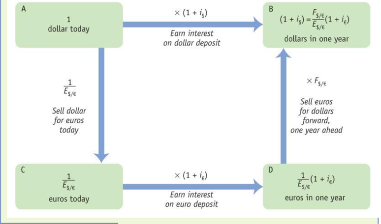
We can rearrange the CIP equation to solve for the forward rate: F$/€=E$/€1+i$1+i€
This equation allows us to calculate the forward rate if we know the spot rate (E$/€), the dollar interest rate (i$), and the euro interest rate (i€). For instance, if the euro interest rate is 3%, the dollar interest rate is 5%, and the spot rate is $1.30 per euro, then the forward rate would be calculated as $1.30 × (1.05)/(1.03) = $1.3252 per euro.
In practice, traders worldwide use this approach to set the price of forward contracts. By observing interest rates on bank deposits in each currency and the spot exchange rate, traders can calculate the forward rate. This process highlights why forward contracts are considered "derivative" contracts—their pricing is derived from the underlying spot contract, incorporating additional information on interest rates.
This leads us to a crucial question: How are interest rates and the spot rate determined? We'll explore this question shortly after examining evidence to confirm that covered interest parity indeed holds.
Top of Form
Bottom of Form
Uncovered Interest Parity (UIP) »
The alternative approach to engaging in arbitrage involves using spot contracts and accepting the risk associated with future exchange rates. By exploring this method, we can gain insight into how exchange rates are determined in the spot market.
Imagine you're trading for a bank in New York and must decide whether to invest $1 in a dollar or euro bank deposit for one year. This time, you're using spot contracts only and not hedging against the risk of future exchange rates.
If you invest in a dollar deposit, your $1 will be worth (1 + i$) in one year, representing the dollar return, as before.
On the other hand, if you invest in a euro deposit, your $1 will be converted to euros at the spot rate today, resulting in 1/E$/€ euros. With interest, these euros will be worth (1 + i€)/E$/€ euros in one year. However, you'll need to convert these euros back into dollars using a spot contract at the prevailing exchange rate, which is forecasted as E$/€e, the expected exchange rate.
Based on this forecast, you expect that the (1 + i€)/E euros you'll have in one year will be worth (1 + i€)E$/€e/E dollars. This represents the expected dollar return on euro deposits.
In essence, traders like you face exchange rate risk and must make forecasts of future spot rates to assess their expected returns accurately. This method, known as Uncovered Interest Parity (UIP), considers the expected returns of bank deposits in different currencies without hedging against exchange rate risk.
Uncovered interest parity (UIP) provides a theory of what determines the spot exchange rate, as it establishes an equilibrium where investors are indifferent between the returns on unhedged interest-bearing bank deposits in two currencies, without the use of forward contracts.
We can rearrange the UIP equation and solve for the spot rate: E$/€=E$/€e1+i€1+i$
- This equation tells us that if uncovered interest parity holds, today's spot rate can be calculated if we know the expected future exchange rate (E$/€e), the dollar interest rate (i$), and the euro interest rate (i€).
EX: if the euro interest rate is 2%, the dollar interest rate is 4%, and the expected future spot rate is $1.40 per euro, then today's spot rate would be 1.40×1.021.04=$1.37311.40×1.041.02=$1.3731 per euro.
However, this leads to more questions: How can the expected future exchange rate (E$/€e) be forecasted? And how are the two interest rates (i$ and i€) determined?
In the following chapters, we'll delve into these questions to further develop our understanding of exchange rate determination. We'll explore the determinants of the expected future exchange rate (�$/€�E$/€e) and develop a model of exchange rates in the long run. Additionally, we'll examine the determinants of the interest rates (i$ and i€). Understanding these concepts is crucial for comprehending exchange rates both in the long run and the short run.
Evidence on Uncovered Interest Parity (UIP)
Uncovered interest parity (UIP) and covered interest parity (CIP) are two similar yet distinct concepts that describe equilibrium conditions in the forex market. While CIP uses the forward rate, UIP relies on the expected future spot rate. However, under certain assumptions, both CIP and UIP imply that the forward rate and the expected future spot rate should be equal.
Mathematically, this can be expressed as: F$/€ = E$/€e
Where:
- F$/€ is the forward rate.
- E$/€e is the expected future spot rate.
This equivalence suggests that in equilibrium, investors should be indifferent between using the forward rate or waiting for the future spot rate, assuming they do not consider risk.
Testing UIP involves comparing the forward premium (the difference between the forward and spot rates) with the expected rate of depreciation (the change in the spot rate over time). If UIP holds, the forward premium should equal the expected rate of depreciation.
Forward premium=E$/€F$/€−1
Expected rate of depreciation= E$/€E$/€e−1
If the forward rate equals the expected future spot rate, then the forward premium should equal the expected rate of depreciation.
Empirical tests of UIP involve surveys where forex traders report their expectations. Despite some deviations from the ideal relationship, the overall evidence suggests a strong correlation between the forward premium and the expected rate of depreciation, supporting the concept of UIP. However, deviations may occur due to factors such as sampling errors, market frictions, and risk aversion among traders. Overall, the evidence provides some support for UIP, although it is not without limitations and challenges in real-world applications.
Top of Form
Uncovered Interest Parity (UIP)
provides a fundamental principle in international macroeconomics, offering insight into how the spot exchange rate is determined. However, for practical purposes, a simplified approximation can often suffice.
The concept behind this approximation is straightforward: Holding dollar deposits earns dollar interest, while holding euro deposits provides euro interest and potential gains or losses due to changes in the euro's value relative to the dollar. To maintain investor indifference between dollar and euro deposits, any shortfall in euro interest must be compensated by an expected gain from euro appreciation or dollar depreciation.
Formally, the UIP approximation equation is expressed as follows:
∆E$/€e/E$/€ = (E$/€e − E$/€)/E$/€
Where:
- i$ is the interest rate on dollar deposits.
- i€ is the interest rate on euro deposits.
- Δ$/€$/€E$/€ΔE$/€e represents the expected rate of change in the euro's value relative to the dollar, which approximates the expected rate of dollar depreciation.
This equation states that the home interest rate equals the foreign interest rate plus the expected rate of depreciation of the home currency.
EX: Suppose the dollar interest rate is 4% per year and the euro interest rate is 3% per year. To uphold UIP, the expected rate of dollar depreciation over a year should be 1%. In this scenario, a dollar investment converted into euros would grow by 3% due to euro interest, plus an additional 1% due to euro appreciation. Thus, the total dollar return on the euro deposit approximates the 4% offered by dollar deposits.
In summary, whether in its exact form or its simplified approximation, uncovered interest parity dictates that expected returns, when expressed in a common currency, should be equal across different markets.
Top of Form
Bottom of Form
Bottom of Form
Chapter 14 : Exchange Rates I: The Monetary Approach in the Long Run
14.1. Exchange rates + prices in the LR
Arbitrage not only occurs in international markets for financial assets but also international markets for goods .
The law of one price
The Law of One Price (LOOP) basically says that identical goods sold in different places should have the same price when you compare those prices in a common currency, assuming there are no barriers like transportation costs or tariffs.
EX: Suppose diamonds of the same quality are priced at €5,000 in Amsterdam, and the exchange rate is $1.20 per euro. According to LOOP, if we convert the euro price to dollars, it should be the same as the price of diamonds in New York.
Here's why prices should be the same:
- If diamonds were cheaper in New York, people would buy them there and sell them in Amsterdam for a profit.
- If diamonds were cheaper in Amsterdam, people would buy them there and sell them in New York for a profit.
LOOP ensures that there are no such profitable opportunities because arbitrage (buying low and selling high) keeps prices aligned across markets.
 Mathematically, we can express LOOP as the ratio of the price of a good in one location to its price in another location, both in the same currency. If this ratio equals 1, it means prices are the same in both places.
P![]() : good’s price in the U.S. P
: good’s price in the U.S. P![]() : good’s price in Europe.
: good’s price in Europe.
q![]() : the rate at which goods can be exchanged.
: the rate at which goods can be exchanged.
E![]() : the rate at which the currencies of the two countries can be exchanged.
: the rate at which the currencies of the two countries can be exchanged.
The law of one price is essential in understanding exchange rates. If it holds true, it means that the exchange rate should be equal to the ratio of prices of goods in two countries when expressed in their respective currencies.
Purchasing power parity
Purchasing Power Parity (PPP) is like the big sibling of the Law of One Price. While the Law of One Price focuses on comparing the prices of single goods across different locations, PPP looks at the prices of entire baskets of goods.
Here's a breakdown of PPP:
- Price Level:
- We define a price level (P) in each location as an average of prices for all goods in a basket, using the same goods and weights in both places.
- Let's call the basket's price in the United States PUS and in Europe PEUR. If the Law of One Price holds for each good in the basket, it will also hold for the basket's overall price.
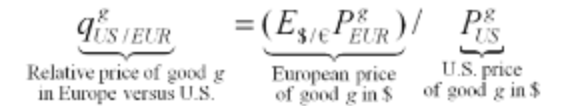
- Relative Price (qUS/EUR):
- We calculate the relative price of the two baskets of goods in each location, denoted qUS/EUR.
- This relative price tells us how the basket's price in Europe compares to its price in the United States when expressed in a common currency (like dollars).
- Possible Outcomes:
- Similar to the Law of One Price, there are three outcomes for PPP:
- The basket is cheaper in the United States.
- The basket is cheaper in Europe.
- The basket costs the same in both locations (qUS/EUR = 1).
- Only when the basket costs the same in both places is there no opportunity for profitable arbitrage. This is when PPP holds true.
- Similar to the Law of One Price, there are three outcomes for PPP:
EX: the European basket costs €100, and the exchange rate is $1.20 per euro.
- For PPP to hold, the U.S. basket would have to cost $120 (1.20 × €100).
In summary, PPP states that price levels in different countries should be equal when expressed in a common currency. This concept is crucial in understanding how exchange rates and price levels interact on a broader scale.
Top of Form
The real exchange rate Bottom of Form
The Real Exchange Rate (q) is like the big sibling of the relative price of individual goods (qg). It tells us how many baskets of goods from one country are needed to purchase one basket from another country.
Here's a breakdown of the Real Exchange Rate:
- Definition:
- The real exchange rate qUS/EUR = E$/€PEUR = PUS tells us how many U.S. baskets are needed to buy one European basket.
- It's a macroeconomic concept that focuses on comparing the overall prices of baskets of goods between countries.
- Understanding the Numerator and Denominator:
- In our example, qUS/EUR = E$/€PEUR = PUS is called the home country or U.S. real exchange rate. It represents the price of the European basket in terms of the U.S. basket.
- It's important to distinguish between nominal exchange rates (like how many dollars for one euro) and real exchange rates (like how many U.S. baskets for one European basket).
- Terminology:
- Similar to nominal exchange rates, we have terminology for changes in real exchange rates:
- If the real exchange rate rises (more U.S. baskets are needed for one European basket), it's called a real depreciation for the home country.
- If the real exchange rate falls (fewer U.S. baskets are needed for one European basket), it's called a real appreciation for the home country.
- Similar to nominal exchange rates, we have terminology for changes in real exchange rates:
In simple terms, the Real Exchange Rate helps us understand how the prices of baskets of goods in different countries relate to each other. If more U.S. goods are needed to buy one European basket, it's a sign of real depreciation for the U.S. Conversely, if fewer U.S. goods are needed, it's a sign of real appreciation.
Absolute ppp and the real exchange rate
Absolute Purchasing Power Parity (PPP) states that the real exchange rate equals 1. This means that all baskets of goods should have the same price when expressed in a common currency, making their relative price 1.
When the real exchange rate is below 1, it means that foreign goods are relatively cheap compared to home goods. In this case:
- The home currency (like the dollar) is considered strong.
- The foreign currency (like the euro) is considered weak.
- We say that the foreign currency is undervalued by a certain percentage (x%).
Conversely, when the real exchange rate is above 1, it means that foreign goods are relatively expensive compared to home goods. In this case:
- The home currency is considered weak.
- The foreign currency is considered strong.
- We say that the foreign currency is overvalued by a certain percentage (x%).
EX: If a European basket costs $550 in dollar terms and a U.S. basket costs $500, then the real exchange rate qUS/EUR = E$/€PEUR / PUS = $550 / $500 = 1.10.
In this case, the euro is strong, and it's considered to be overvalued against the dollar by 10%
Absolute PPP, Prices, and the Nominal Exchange Rate
Absolute Purchasing Power Parity (PPP) provides a straightforward prediction about exchange rates: the exchange rate between two currencies should be equal to the ratio of the price levels in the two countries.
Absolute PPP: E€/$ = PUS / PEUR
- This equation tells us that the exchange rate (E$) between the dollar and the euro equals the ratio of price levels (PUS and PEUR) in the United States and Europe, respectively.
EX: If a basket of goods costs $500 in the United States and €400 in Europe, the theory of PPP predicts an exchange rate of $500/€400 = $1.25 per euro.
So, if we know the price levels in different locations, we can use PPP to determine an implied exchange rate. This relationship is crucial in understanding how exchange rates are determined. Additionally, PPP can help forecast future exchange rates based on forecasted future price levels.
In summary, Absolute PPP is a fundamental concept in understanding how exchange rates are determined, and it provides valuable insights into the relationship between price levels and exchange rates.
Relative PPP , inflation & exchange rate depreciation
Relative Purchasing Power Parity (PPP) focuses on the relationship between changes in prices and changes in exchange rates, rather than the absolute levels of prices and exchange rates.
Here's how it works:
- Inflation and Exchange Rate Depreciation:
- In macroeconomics, we're often more interested in how price levels change over time. The rate of growth of the price level is known as inflation.
- Relative PPP states that the rate of depreciation of the nominal exchange rate (the change in the exchange rate over time) equals the difference between the inflation rates of two countries (the inflation differential).
- Equation for Relative PPP:
- Relative PPP is described by the equation: ΔE$/€ / E$/€=Inflation differential
- This equation shows that the rate of depreciation of the nominal exchange rate equals the difference between the inflation rates of two countries.
Example: if Canadian prices rose 16% more than U.S. prices over 20 years, and the Canadian dollar depreciated 16% against the U.S. dollar, then relative PPP held. This translates to an annual inflation differential of 0.75%, with the Canadian dollar depreciating by 0.75% per year against the U.S. dollar.
Relationship with Absolute PPP:
- Relative PPP is derived from absolute PPP. While absolute PPP focuses on the levels of prices and exchange rates, relative PPP focuses on their changes over time.
- Absolute PPP implies relative PPP, but the reverse isn't always true. Relative PPP doesn't necessarily imply absolute PPP. For example, relative PPP can hold even if absolute PPP fails, as long as the inflation differential matches the rate of depreciation.
In summary, both forms of Purchasing Power Parity suggest a tight link between price levels in different countries and exchange rates, either in their absolute levels or in their rates of change over time
Evidence for PPP in the Long Run and Short Run
Evidence for Purchasing Power Parity (PPP) varies depending on the time horizon:
- Long Run Evidence (Relative PPP):
- Over long periods, such as decades, there is some support for relative PPP.
- Data from a sample of countries over three decades (1975-2005) show a strong correlation between the rate of exchange rate depreciation against the U.S. dollar and the inflation differential against the United States.
- While not exact, the data generally align with the theoretical prediction of PPP, indicating that relative PPP serves as an approximate guide to the relationship between prices and exchange rates over the long run.
- Short Run Evidence (Absolute and Relative PPP):
- In the short run, typically spanning just a few years, evidence for both absolute and relative PPP is weak.
- Time series data for specific pairs of countries, such as the United States and the United Kingdom from 1975 to 2010, show substantial and persistent differences between the relative price ratio and exchange rates from year to year.
- While relative price levels tend to change slowly with a small range of movement, exchange rates experience larger and more abrupt fluctuations.
- Absolute and relative PPP fail in the short run, as evidenced by significant differences in levels and changes between relative price ratios and exchange rates, even over periods of several years.
In summary, while relative PPP provides a useful guide to the relationship between prices and exchange rates over the long run, absolute and relative PPP tend to fail in the short run, where significant fluctuations and deviations from theoretical predictions are observed.
How slow is convergence to PPP
Convergence to Purchasing Power Parity (PPP) is not immediate; rather, it occurs gradually over time. Research indicates that price differences, or deviations from PPP, persist for a considerable period.
- Estimates suggest that these deviations diminish at a rate of approximately 15% per year. This means that after one year, 85% of the initial price difference still remains, and after four years, about 52% of the deviation persists.
- Economists often refer to this rate of convergence as a "half-life." For instance, a four-year half-life implies that after four years, approximately half of the initial deviation from PPP still exists.
These estimates serve as a useful rule of thumb for forecasting real exchange rates. For example, if the home basket costs $100 and the foreign basket costs $90 in home currency, indicating that the home currency is overvalued, the deviation of the real exchange rate from the PPP-implied level is calculated.
- Using the rule of thumb, one can forecast that 15% of this deviation will disappear in the next year, leading to a new forecast deviation.
- Similarly, after four years, approximately 52% of the deviation would have been erased, bringing the real exchange rate closer to the PPP level.
Overall, these estimates help economists anticipate how deviations from PPP are expected to change over time, providing insights into the movement of real exchange rates
What explains deviations from PPP ?
Deviation from Purchasing Power Parity (PPP) can be explained by several factors:
- Transaction costs: Trade is not completely frictionless due to significant costs associated with international transportation and additional expenses like tariffs and duties. These costs can add up to around 20% for transportation and 10% for tariffs, making arbitrage less efficient and slowing down the adjustment of prices across borders.
- Nontraded goods: Some goods are inherently nontradable due to high transaction costs, which hinders arbitrage and prevents PPP from holding. Most goods and services fall between tradable and nontradable categories, complicating the application of PPP.
- Imperfect competition and legal obstacles: Many goods are not simple commodities but differentiated products with brand names and legal protections. Firms may have the power to set prices differently across countries, and legal threats or regulations can prevent arbitrage activities. This imperfect competition can lead to price differences across borders.
- Price stickiness: Prices are often sticky in the short run, meaning they do not adjust quickly to changes in market conditions. While PPP assumes that arbitrage will force prices to adjust, price stickiness slows down this adjustment process, causing deviations from PPP.
Despite these challenges, PPP remains a useful long-run theory of exchange rates. As globalization continues and arbitrage becomes more efficient, PPP may become even more relevant in the future. The increasing trade of goods and services, along with advancements in technology and communication, could lead to more efficient arbitrage and a closer alignment of prices across borders.
When PPP doesn't hold, forecasting exchange rate changes requires estimating the current level of the real exchange rate and the convergence speed towards absolute PPP in the long run. Here's how you can construct a forecast of real and nominal exchange rates:
- Start with the definition of the real exchange rate: qUS/EUR= E$/\€. / PEUR/PUS
- Rearrange the equation to find the nominal exchange rate (E$/\€): qUS/EUR × PUS / PEUR
- By taking the rate of change of the above expression, you find that the rate of change of the nominal exchange rate equals the rate of change of the real exchange rate plus home inflation minus foreign inflation:
- If the real exchange rate (q) is constant, the first term on the right is zero, and you're back to the simple world of relative PPP, where the predicted nominal depreciation is just the inflation differential.
- However, if �q isn't constant and PPP fails, you need to estimate the rate of convergence towards absolute PPP. Suppose you're given that a U.S. basket of goods currently costs $100, but the European basket of the same goods costs $130, giving a U.S. real exchange rate of 1.30. If you expect absolute PPP to hold in the long run, you expect the U.S. real exchange rate to move toward 1. Using the 15% rule of thumb, you estimate that 15% of the 0.3 gap between 1 and 1.3 (i.e., 0.045) will dissipate over the coming year. Therefore, you forecast that the U.S. real exchange rate will fall from 1.3 to 1.255, implying a change of -3.46% in the coming year.
- Adding the rate of depreciation of the real exchange rate (-3.46%) to the inflation differential (+2%), you get a total of -1.46%. This suggests a dollar appreciation of 1.46% against the euro.
This forecast considers both the expected convergence of the real exchange rate towards absolute PPP and the inflation differentials between the two countries.
14.2 Money prices and exchange rates in the long run
What is money ?
Money is a fundamental concept in economics, serving three key functions:
- Store of Value: Money allows ppl to store purchasing power over time. Despite not yielding interest, money retains its value and can be used to buy goods and services in the future. While other assets may offer higher returns, money's liquidity and stability make it a preferred choice for storing value, especially for short-term needs.
- Unit of Account: Money serves as a common measure for expressing the value of goods and services in an economy. Prices are quoted in terms of the currency unit, providing a standard measure that facilitates economic transactions and comparisons. While other items could potentially serve as units of account, money's widespread acceptance and stability make it the preferred choice.
- Medium of Exchange: Money facilitates the exchange of goods and services by eliminating the need for direct barter, where individuals would have to trade goods for goods. Money enables transactions to occur efficiently, as it is universally accepted and highly liquid. Its widespread acceptance and ease of use make money the primary medium of exchange in modern economies.
These three functions make money a cornerstone of economic activity, enabling individuals to store value, measure economic transactions, and facilitate the exchange of goods and services. Despite its simplicity, the role of money is essential for the functioning of modern economies.
Meausrment of money
The measurement of money encompasses various financial instruments, each representing different degrees of liquidity and suitability for transactions. Here's an overview of the main categories:
- Currency in Circulation: This refers to physical coins and banknotes held by the nonbank public. It is the most basic form of money and serves as a medium of exchange in everyday transactions.
- M0: Also known as base money, M0 includes currency in circulation and the reserves held by commercial banks. Typically, bank reserves are minimal, so M0 is often equivalent to currency in circulation. However, during times of financial crisis, banks may accumulate significant reserves as a precautionary measure.
- M1: This narrow measure of money includes currency in circulation and demand deposits in checking accounts. It represents the most liquid assets readily available for transactions, excluding bank reserves.
- M2: A broader measure of money, M2 includes M1 plus slightly less liquid assets such as savings deposits and small time deposits. While still relatively liquid, these assets may not be as readily available for transactions as those included in M1.
In summary, money can be defined as the stock of liquid assets routinely used for transactions. In this context, M1, which comprises currency in circulation and demand deposits, is often considered the primary measure of money for practical purposes. Assets excluded from M1, such as longer-term investments and interbank deposits, are not typically used as mediums of exchange in day-to-day transactions due to their relative illiquidity.
The supply of money
The supply of money is primarily determined by the country's central bank, which has direct control over the level of base money (M0) and indirect influence over broader measures of money like M1. Here's how it works:
- Direct Control over M0: The central bank directly controls the amount of currency (notes and coins) in circulation and the reserves held by commercial banks. By issuing or withdrawing currency and adjusting reserve requirements, the central bank can directly influence the level of M0 in the economy.
- Indirect Control over M1: While the central bank's direct control is limited to M0, it can indirectly affect broader measures of money such as M1. This is achieved through monetary policy tools, such as open market operations, discount rate changes, and reserve requirement adjustments. By influencing interest rates, credit availability, and the behavior of commercial banks, the central bank can impact the creation of bank deposits, thus affecting the overall level of M1.
In practice, the central bank's goal is to use monetary policy to achieve macroeconomic objectives such as price stability, full employment, and economic growth. While the mechanisms by which monetary policy affects M1 are complex and multifaceted, the central bank's policy tools are designed to provide sufficient control over the money supply, allowing it to approximate the desired level of M1 indirectly.
Top of Form
Bottom of Form
The demand for money : a simple modelTop of Form
Bottom of Form
The demand for money can be understood through a simple model known as the quantity theory of money. This theory suggests that the demand for money is proportional to nominal income. Here's a breakdown of the model:
- Basic Model: The demand for money (Md) is determined by a constant factor (L ̄) multiplied by the total nominal income (PY) in the economy. The term PY represents the total nominal value of income, where P is the price level and Y is the real income.
- Constant Factor: The constant factor (L ̄) represents how much demand for liquidity is generated for each dollar of nominal income. It's assumed that every dollar of nominal income requires a certain amount of money for transactions purposes, and this relationship is constant.
- Intuition: If the price level rises (inflation), the dollar cost of transactions increases proportionally, leading to higher demand for money. Similarly, if real income increases, the volume of transactions also increases, leading to higher demand for money.
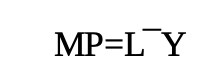 Real Money Balances: Another perspective is to consider real money balances, which measure the purchasing power of money in terms of goods and services. Dividing the basic equation by the price level (P) yields the demand for real money balances. In this case, the demand for real money balances is proportional to real income (Y). More real income implies more real transactions, requiring more real money.
In summary, the quantity theory of money suggests that the demand for money is linked to nominal income, with variations in inflation and real income affecting the demand for money accordingly.
Top of Form
A simple monetary model of prices Bottom of Form
This simple monetary model of prices helps us understand how the price level in each country is determined by monetary conditions. Here's how the model works:
- Quantity Theory Equation: The model begins with the quantity theory equation, which relates the price level (P) to the money supply (M) and the demand for real money balances (L ̄Y). For the United States (US), the equation is P_{US} = \frac{M_{US}}{L ̄_{US}Y_{US}}. Similarly, for the Eurozone (EUR), the equation is P_{EUR} = \frac{M_{EUR}}{L ̄_{EUR}Y_{EUR}}.
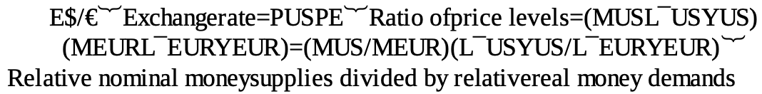
- Money Supply and Real Income: In these equations, the money supply (M) and real income (Y) are treated as exogenous variables, meaning they are assumed to be known and fixed. The money supply represents the total amount of money issued by the central bank, while real income reflects the total output of goods and services in the economy.
- Demand for Real Money Balances: The demand for real money balances (L ̄Y) represents the amount of money individuals and businesses wish to hold for transactions purposes relative to real income. It captures the need for liquidity in the economy.
- Price Level Determination: The price level in each country is determined by the ratio of the money supply to the demand for real money balances. If the money supply increases relative to the demand for money, it leads to "more money chasing the same quantity of goods," resulting in inflation. In the long run, prices adjust to put the money market in equilibrium, with the price level rising proportionally to changes in the money supply.
- Flexibility of Prices: In the long run, prices are assumed to be flexible, allowing them to adjust to changes in monetary conditions. For example, if the money supply increases significantly while real income remains constant, prices will rise to restore equilibrium in the money market.
Overall, this model provides a framework for understanding how monetary factors influence the price level in each country over the long run.
A simple monetary of the exchange rate
This simple monetary model of the exchange rate combines the quantity theory of money and purchasing power parity (PPP) to explain how changes in monetary and real economic conditions affect the exchange rate between two countries. Here's how the model works:
- Equation Setup: We start by plugging the price levels derived from the monetary model into the PPP equation E$/€=PUS/ PEUR .
- Impact of Changes in Money Supply: If the U.S. money supply increases, while all else remains constant, the right-hand side of the equation increases. This means that the U.S. nominal money supply increases relative to Europe, causing the exchange rate (E$/€) to increase. In other words, the U.S. dollar depreciates against the euro. This makes sense intuitively because with more dollars in circulation, each dollar becomes less valuable.
- Impact of Changes in Real Income: If the U.S. real income level increases, while all else remains constant, the right-hand side of the equation decreases. This indicates that the U.S. real money demand increases relative to Europe, causing the exchange rate (E$/€) to decrease. In this scenario, the U.S. dollar appreciates against the euro. A stronger U.S. economy leads to higher demand for dollars, making each dollar more valuable.
Overall, this model provides insights into how changes in monetary and real economic factors influence the exchange rate between two countries. It shows that both the money supply and real income levels play significant roles in determining the value of a country's currency relative to another.
Top of Form
Money , growth and deprieciation ??????Bottom of Form
Equation (14-6) provides a framework for understanding how changes in monetary policy and real economic conditions affect inflation differentials and, consequently, the rate of depreciation of the exchange rate. Here's a breakdown of how it works:
- Understanding the Equation: Equation (14-6) expresses the rate of depreciation of the nominal exchange rate (Δ�$/€/�$/€ΔE$/€/E$/€) as the difference between the inflation differentials of the two countries. This differential is then decomposed into two components: the differential in nominal money supply growth rates and the differential in real output growth rates.
- Impact of Monetary Policy: If one country adopts a looser monetary policy, characterized by a faster growth rate of the money supply, it will experience higher inflation. Conversely, a tighter monetary policy leads to lower inflation. For example, if the U.S. increases its money supply by 6% annually while Europe increases it by only 5%, and both have the same real income growth rate of 2%, the inflation differential would be 1%. This differential influences the rate of depreciation of the dollar against the euro.
- Impact of Real Economic Growth: Changes in real output growth rates also affect inflation differentials. If one country experiences faster economic growth, it may lead to lower inflation if the growth outpaces the increase in the money supply. For instance, if the U.S. real income growth rate increases from 2% to 5% annually, and all else remains equal, the inflation differential would be affected accordingly. If U.S. inflation becomes lower than European inflation, the dollar may appreciate against the euro.
- Lessons for Exchange Rate Dynamics: These examples demonstrate that changes in monetary policy and real economic conditions influence inflation and, subsequently, the exchange rate dynamics between two countries. A looser monetary policy or faster real economic growth in one country relative to another tends to lead to currency depreciation, while tighter monetary policy or slower real economic growth may result in currency appreciation.
By analyzing these factors, economists can gain insights into how changes in policy and economic conditions impact exchange rates and make predictions about future exchange rate movements.
Top of Form
14.3. the monetary approach : implications & evidenceBottom of Form
Exchange rate forecasts using the simple model.
The monetary approach to exchange rate determination provides a framework for forecasting future exchange rate movements based on expectations about money supplies and real income. Let's delve into the process of forecasting exchange rates using the simple model presented:
- Forecasting Methodology: Equation (14-3) serves as the foundation for forecasting future exchange rates. It links the future exchange rate (left-hand side) with expectations about future money supplies and real income (right-hand side). Therefore, forecasts rely heavily on predictions about central bank policies and economic growth.
- Attention to Economic Indicators: Forecasts of money supplies and real income attract significant attention in financial markets and the forex market. Analysts closely monitor central bank statements and economic indicators to anticipate changes in monetary policy and economic conditions. Any insights into future policy actions or economic trends can inform exchange rate forecasts.
- Caveats and Uncertainty: Forecasting future economic variables, including money supplies and real income, is inherently uncertain. Predictions made years in advance are prone to large errors due to unforeseen events and changes in economic conditions. Despite this uncertainty, financial markets rely on these forecasts for decision-making.
- Hypothetical Assumptions: It's important to recognize that using the monetary model for forecasting entails making hypothetical assumptions. Forecasts are based on the premise that prices are flexible, and purchasing power parity holds. While short-term deviations may occur, the model provides a reasonable guide for longer-term exchange rate movements.
To illustrate how forecasting works, let's consider two hypothetical scenarios:
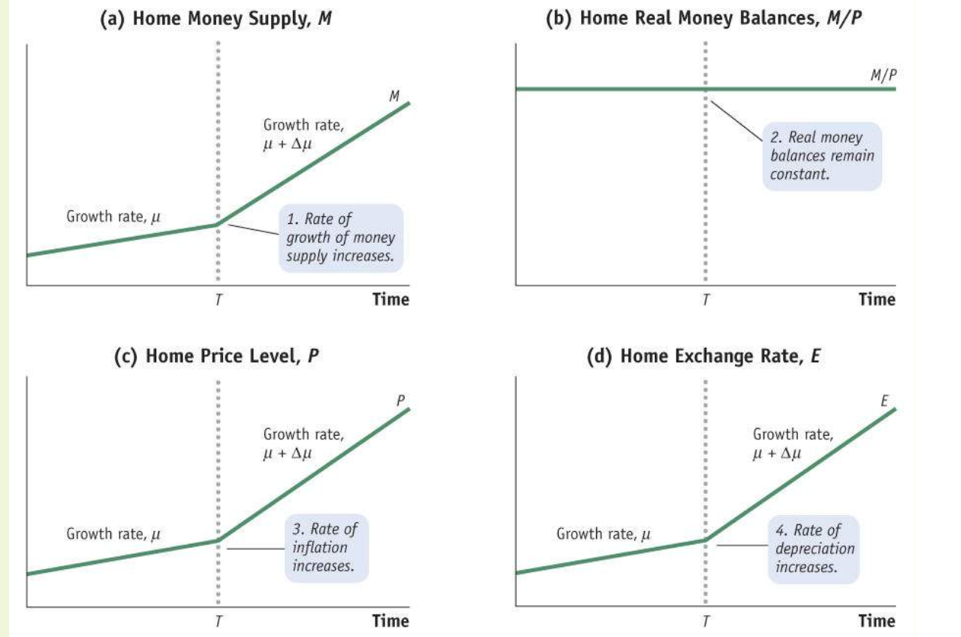 Case 1: One-time Increase in Money Supply: If the U.S. money supply unexpectedly increases by 10% at a certain time, assuming constant real income levels, the model predicts a corresponding 10% increase in the price level and, consequently, a 10% depreciation of the dollar against the euro.
- Case 2: Increase in Money Supply Growth Rate: In another scenario, if the U.S. money supply grows at a constant rate initially and then increases to a slightly higher rate, the model predicts a proportional increase in prices and the exchange rate. This increase in the rate of money supply growth leads to higher inflation and depreciation of the dollar against the euro.
These examples demonstrate how changes in monetary policy and economic conditions affect exchange rate forecasts according to the monetary approach. By analyzing the relationships between money supplies, real income, prices, and exchange rates, economists and market participants can make informed predictions about future currency movements.
Evidence for the monetary apporach
The evidence presented in the scatterplots from 1975 to 2005 provides support for the monetary approach to prices and exchange rates. Here's a breakdown of the findings and their implications:
- Relationship Between Money Supply Growth, Inflation, and Exchange Rate Depreciation: The scatterplots illustrate the relationship between the rate of money supply growth, inflation rates, and exchange rate depreciation across a large sample of countries. According to Equation (14-6), increases in the rate of money supply growth should correspond to similar increases in inflation rates and exchange rate depreciation.
- Expected Relationship: In an ideal scenario where all else is equal, each country's data point on the scatterplot would align closely with the 45-degree line. This alignment would indicate a direct association between the percentage difference in money supply growth rates, inflation rates, and exchange rate depreciation relative to the United States.
- Close Relationship in Data: While not every data point aligns perfectly with the 45-degree line, the actual relationship observed in the scatterplots closely resembles the expected pattern. This alignment provides empirical support for the monetary approach, suggesting that variations in money supply growth rates are indeed associated with similar variations in inflation rates and exchange rate depreciation across countries.
- Factors Affecting Deviation: Deviations from the ideal alignment can be attributed to several factors. Firstly, countries in the sample may differ not only in their relative money supply growth rates but also in their real income growth rates. Additionally, assumptions such as the constant parameter L in Equation (14-6) may not hold true in reality, contributing to discrepancies between predicted and observed outcomes.
Overall, while the evidence from the scatterplots supports the monetary approach to prices and exchange rates, it also highlights the need to consider additional factors and potential deviations from theoretical predictions when analyzing real-world data.
Hyperinflations provide a unique scenario for testing the validity of the purchasing power parity (PPP) theory. Here's a summary of the key points regarding PPP in hyperinflations:
- Definition of Hyperinflation: Hyperinflation is traditionally defined as a sustained period during which the inflation rate exceeds 50% per month. Such extreme inflation results in prices doubling every few days, leading to significant economic, social, and political crises.
- PPP in Hyperinflations: Despite the generally poor performance of PPP in the short run, hyperinflations serve as an exception. During hyperinflations, PPP tends to hold quite well, even in the short term. This means that changes in prices and exchange rates are closely correlated and follow the same pattern.
- Scatterplot Analysis: Scatterplots, such as the one depicted in Figure 14-9, illustrate the relationship between the cumulative start-to-finish exchange rate depreciation against the U.S. dollar and the cumulative start-to-finish rise in the local price level during hyperinflations. The data points align closely with the theoretical prediction of PPP, indicating a strong correlation between changes in prices and exchange rates.
- Evidence of Extreme Changes: The logarithmic scales used in the scatterplots highlight the extreme changes involved in hyperinflations. For instance, a value of 10^12 on the vertical axis represents a trillion-fold increase in the exchange rate against the U.S. dollar.
- Causes of Hyperinflations: Hyperinflations typically occur due to governments facing budget crises and resorting to printing money to finance deficits. This unsustainable practice leads to rapid depreciation of the currency and soaring inflation rates.
- Collapse of Real Money Balances: During hyperinflations, real money balances tend to collapse as people minimize their holdings of rapidly depreciating currency. The higher the inflation rate, the lower the level of real money balances, reflecting the practical behavior of individuals in response to hyperinflationary pressures.
Overall, hyperinflations serve as a unique laboratory for testing PPP theory, demonstrating its validity even in extreme economic conditions characterized by rapidly changing prices and exchange rates.
14.4 Money , interest rates and prices in LR : Genreal model
we aim to refine our understanding of the long-run relationship between money, interest rates, and prices by developing a more comprehensive model that addresses the shortcomings of the quantity theory. While the quantity theory assumes a stable demand for money, which may not hold true in reality, we seek to incorporate variations in money demand by introducing the nominal interest rate as a determinant.
To accomplish this, we need to explore how the nominal interest rate is determined in the long run within an open economy framework.
The general model of money demand builds upon the insights from the quantity theory, incorporating both the benefits and costs of holding money. At the individual level, holding money allows for transactions but incurs an opportunity cost in terms of foregone interest earnings. Extrapolating to the macroeconomic level, we can infer that aggregate money demand will increase with nominal income but decrease with the nominal interest rate.
This leads us to a general model where money demand is proportional to nominal income and is inversely related to the nominal interest rate. Mathematically, this relationship can be expressed as:
��=�(�)×�×�Md=L(i)×P×Y
where:
- ��Md represents the demand for money in dollars,
- �(�)L(i) is a decreasing function representing the liquidity preference, which varies inversely with the nominal interest rate �i,
- �P denotes the price level, and
- �Y signifies nominal income.
To examine the demand for real money balances, we divide by �P to derive:
���=�(�)×�PMd=L(i)×Y
Here, ���PMd represents the demand for real money balances, and �Y stands for real income.
Figure 14-11(a) illustrates a typical real money demand function, with the quantity of real money balances demanded on the horizontal axis and the nominal interest rate on the vertical axis. The downward slope of the demand curve reflects the inverse relationship between the demand for real money balances and the nominal interest rate at a given level of real income �Y.
Figure 14-11(b) demonstrates the effect of an increase in real income from �1Y1 to �2Y2. As real income rises, the demand for real money balances increases at each level of the nominal interest rate, leading to a shift in the demand curve.
Top of Form
The general model of money demand is a framework used in macroeconomics to understand how individuals and firms make decisions about how much money to hold. It builds upon the basic principles of the quantity theory of money but incorporates additional factors to provide a more nuanced understanding of money demand.
Here's what the general model consists of and its purpose:
- Components of the Model:
- Transactions Demand for Money: Money is held to facilitate transactions in the economy. Individuals and firms need money to make purchases of goods and services, pay bills, and conduct everyday transactions.
- Opportunity Cost of Holding Money: Holding money also incurs an opportunity cost. Instead of holding money, individuals could invest in interest-bearing assets such as bonds or savings accounts and earn interest income. Therefore, there is a cost associated with holding money in terms of foregone interest earnings.
- Purpose of the Model:
- Understanding Money Demand: The general model aims to explain why individuals and firms hold money and how their demand for money varies with changes in economic conditions such as income levels and interest rates.
- Policy Implications: By understanding the determinants of money demand, policymakers can make informed decisions about monetary policy. For example, central banks may adjust interest rates or the money supply to influence money demand and thereby stabilize the economy.
- Market Analysis: The model also provides insights into how changes in monetary policy or economic conditions affect financial markets. For instance, changes in interest rates can impact bond prices and stock markets, influencing investor behavior and asset prices.
Overall, the general model of money demand helps economists and policymakers understand the complex relationship between money, interest rates, and economic activity, providing valuable insights into the functioning of modern economies.
Top of Form
LR eq in the money market
In the long-run equilibrium of the money market, the real money supply (determined by the central bank) equals the demand for real money balances (determined by the nominal interest rate and real income). This equilibrium condition is expressed by the equation:
MP=L(i)⋅Y
Where:
- MP represents the real money supply.
- L(i) represents the demand for real money balances as a function of the nominal interest rate i.
- Y represents real income.
This equation indicates that in equilibrium, the quantity of real money supplied by the central bank is equal to the quantity of real money demanded by individuals and firms in the economy.
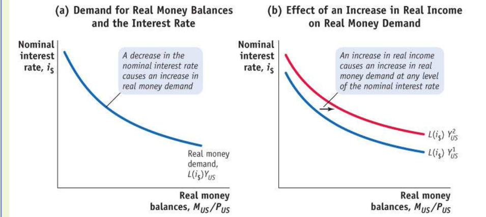 The downward slope of the real money demand function (as shown in Panel (a) of Figure 14-11) implies that as the nominal interest rate decreases, the demand for real money balances increases. Similarly, an increase in real income (as shown in Panel (b) of Figure 14-11) leads to a rise in the demand for real money balances at all levels of the nominal interest rate.
In summary, the long-run equilibrium in the money market occurs when the real money supply equals the demand for real money balances, which depends on the nominal interest rate and real income. This equilibrium condition is crucial for understanding the determination of the exchange rate and other macroeconomic variables in the long run.
Top of Form
Inflation & Interest Rates in the Long Run
In the long run, the relationship between inflation differentials and interest rate differentials in an open economy is determined by two key concepts: Relative Purchasing Power Parity (Relative PPP) and Uncovered Interest Parity (UIP).
Relative PPP, expressed in Equation (14-2), states that the rate of depreciation of the exchange rate equals the inflation differential between two countries at time t. When market participants use this equation to forecast future exchange rates, denoted by the superscript e, it can be rewritten to show the expected depreciation and inflation at time �t:
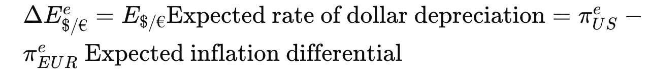
Expected inflation differential
Here, Δ�$/€�ΔE$/€e represents the expected rate of dollar depreciation against the euro, ����πUSe represents the expected inflation rate in the United States, and �����πEURe represents the expected inflation rate in the eurozone.
UIP, in its approximate form as expressed in Equation (13-3), can be rearranged to show that the expected rate of depreciation of the exchange rate equals the interest rate differential between two countries at time t:
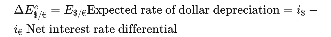
Here, �$i$ represents the net dollar interest rate, and �€i€ represents the net euro interest rate.
This formulation of UIP suggests that traders will be indifferent to a higher U.S. interest rate relative to euro interest rates only if the higher U.S. rate is offset by an expected depreciation of the U.S. dollar against the euro. For example, if the U.S. interest rate is 4% and the euro interest rate is 2%, the interest rate differential is 2%, and the forex market can be in equilibrium only if traders expect a 2% depreciation of the U.S. dollar against the euro to offset the higher U.S. interest rate.
The Fisher Effect
Because the left sides of the previous two equations are equal, the right sides must also be equal. Thus, the nominal interest differential equals the expected inflation differential:
i$−i€Nominal interestrate differential=πUSe−πEURe
Nominal inflation ratedifferential (expected) (14-8)
What does this important result say? To take an example, suppose expected inflation is 4% in the United States and 2% in Europe. The inflation differential on the right is
then +2% (4% − 2% = +2%). If interest rates in Europe are 3%, then to make the interest differential the same as the inflation differential, +2%, the interest rate in the United States must equal 5% (5% − 3% = +2%).
Now suppose expected inflation in the United States changes, rising by one percentage point to 5%. If nothing changes in Europe, then the U.S. interest rate must also rise by one percentage point to 6% for the equation to hold. In general, this equation predicts that changes in the expected rate of inflation will be fully incorporated (one for one) into changes in nominal interest rates.
All else equal, a rise in the expected inflation rate in a country will lead to an equal rise in its nominal interest rate.
This result is known as the Fisher effect, named for the American economist Irving Fisher (1867–1947). Note that because this result depends on an assumption of PPP, it is therefore likely to hold only in the long run.
The Fisher effect makes clear the link between inflation and interest rates under flexible prices, a finding that is widely applicable. For a start, it makes sense of the evidence we just saw on money holdings during hyperinflations (see Figure 14-10). As inflation rises, the Fisher effect tells us that the nominal interest rate i must rise by the same amount; the general model of money demand then tells us that L(i) must fall because it is a decreasing function of i. Thus, for a given level of real income, real money balances must fall as inflation rises.
In other words, the Fisher effect predicts that the change in the opportunity cost of money is equal not just to the change in the nominal interest rate but also to the change in the inflation rate. In times of very high inflation, people should, therefore, want to reduce their money holdings—and they do.
Bottom of Form
Real interest parity
Real Interest Parity (RIP) is a concept in economics that describes the equalization of expected real interest rates across countries in the long run. Here's a breakdown:
- Equation (14-9): Real Interest Parity states that if Purchasing Power Parity (PPP) and Uncovered Interest Parity (UIP) hold, then expected real interest rates are equalized across countries. Mathematically, this is expressed as ���=����rUS=rEUR, where ���rUS represents the expected real interest rate in the United States and ����rEUR represents the expected real interest rate in Europe.
- Implications: RIP suggests that arbitrage opportunities in goods and financial markets will lead to the equalization of real interest rates across countries in the long run. This implies that differences in expected inflation rates between countries will be offset by adjustments in nominal interest rates.
- Long-Run Assumption: RIP is likely to hold only in the long run, as it depends on the assumptions of PPP and UIP, which themselves are long-run concepts. In the short run, various factors may cause deviations from real interest parity.
- Globalization and Economic Convergence: RIP implies that countries integrated into the global capital market will eventually share a common expected real interest rate. This suggests a potential for globalization to lead to convergence in economic outcomes across countries.
- Policy Implications: RIP suggests that policymakers cannot control the long-run expected real interest rate directly. Instead, it is treated as an exogenous variable, denoted as �∗r∗, outside the control of any individual country's policymakers.
- Relationship with Fisher Effect: RIP provides further clarity on the Fisher Effect, showing that in each country, the long-run expected nominal interest rate is equal to the long-run world real interest rate plus the country's expected long-run inflation rate. This relationship highlights how changes in expected inflation rates impact nominal interest rates in the long run.
Top of Form
The evidence presented supports the Fisher Effect and real interest parity, particularly in the long run:
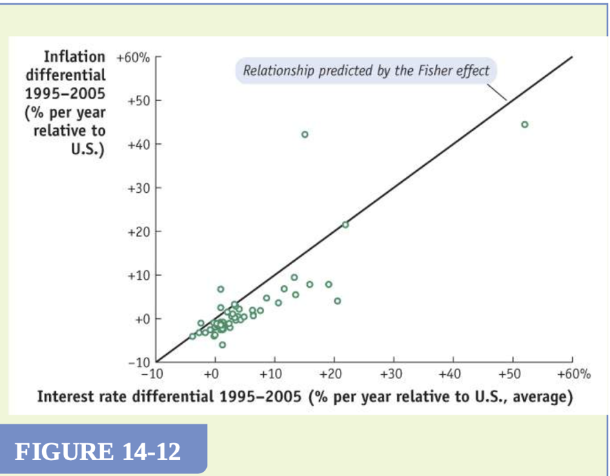 Fisher Effect: The scatterplot in Figure 14-12 illustrates the relationship between the average annual nominal interest rate differential and the annual inflation differential relative to the United States over a ten-year period for a sample of 62 countries. The strong correlation between these variables aligns with the predictions of the Fisher Effect. This suggests that, on average, countries with higher inflation rates tend to have higher nominal interest rates, supporting the Fisher Effect hypothesis.
- Real Interest Parity: Figure 14-13 displays actual real interest rate differentials over four decades for the United Kingdom, Germany, and France relative to the United States. While these differentials were not consistently zero, they fluctuated around zero in the long run. This indicates that while real interest parity did not hold continuously, the differentials were, on average, close to zero. This suggests that real interest parity, similar to PPP, is a general long-run tendency in the data.
Overall, while there may be deviations from these concepts in the short run due to various factors, the evidence suggests that the Fisher Effect and real interest parity hold, at least approximately, in the long run.
Top of Form
Bottom of Form
ChatGPT can make mistakes. Consider checking important information.
Bottom of Form
Chapter 15 – Exchange Rates II: The Asset Approach in the Short Run
The monetary approach to exchange rates focuses on the relationship between money supply, inflation, and exchange rates in the long run. It suggests that changes in money supply and inflation directly impact exchange rates over time.
- aim of the monetary approach is to understand how changes in a country's money supply and inflation rates affect its exchange rate with other currencies over the long term.
However, in the short run, the monetary approach may not fully explain fluctuations in exchange rates. This led economists to develop an alternative theory called the asset approach to exchange rates.
The asset approach looks at exchange rates from the perspective of asset markets, particularly the demand and supply of financial assets like stocks, bonds, and currencies. It considers factors such as investor expectations, interest rates, and risk perceptions.
- The asset approach aims to explain short-term fluctuations in exchange rates by analyzing factors related to asset markets, such as investor expectations, interest rates, and risk perceptions.
So, while the monetary approach emphasizes the role of money supply and inflation in determining exchange rates over the long term, the asset approach complements it by focusing on short-term fluctuations driven by factors related to financial markets and investor behavior.
15.1 Exchange Rates and Interest Rates in the Short run: UIP and FX Market Equilibrium
The equilibrium condition in the FOREX market is a no arbitrage condition { when there are no expected differences in rates of return between investments.Specifically, the dollar rate of return on a home investment (like a dollar deposit) should equal the expected dollar rate of return on a foreign investment (like a euro deposit)}.
Risky Arbitrage
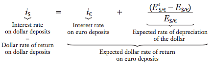 The no-arbitrage condition for risky arbitrage is defined as:
This equation is the UIP, a fundamental equation in the asset approach to exchange rates.
- It states that in equilibrium, the expected return on a foreign investment should equal the domestic interest rate plus the expected rate of depreciation of the domestic currency against the foreign currency. Means that for investors to be indifferent between investing domestically or abroad. The total return expected from investing in a foreign currency should be equal to the return from investing domestically plus any expected gains or losses from changes in the exchange rate between the domestic and foreign currencies.
We will use it to develop our model. Notice that the theory is useful only if we know the future expected exchange rate and the short-term interest rates.
Therefore, we must make two assumptions:
- We know today’s interest rates i on deposit account in each country.
- We know the forecast of the future level of the exchange rate .
Why do we use it ? It helps economists and investors analyze and predict short-term movements in exchange rates based on interest rate differentials between countries. helps determine whether there are arbitrage opportunities in the foreign exchange market
An FX market diagram is a graphical representation of the returns in the forex market. We plot the expected domestic and foreign returns against today’s spot exchange rate. The domestic dollar return is fixed and independent of the spot exchange rate.
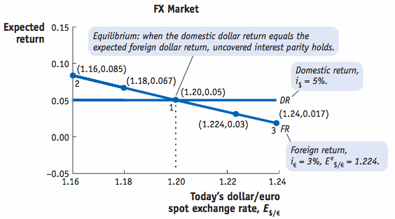 There is one thing that we can observe: the foreign return goes down, all else equal, as the exchange rate rises, so, the foreign return curve will always slope downward.
Why? If the dollar depreciates today, rises; a euro investment is then a more expensive (and, thus, less attractive) proposition, all else equal. That is, $1 moved into a euro account is worth fewer euros today; this, in turn, leaves fewer euro proceeds in a year’s time after euro interest has accrued. If expectations are fixed so that the future euro-dollar exchange rate is known and unchanged, then those fewer future euros will be worth fewer future dollars.
- Dollar Depreciation:
- When the dollar depreciates, it means that it becomes weaker relative to the euro. In other words, you need more dollars to buy the same amount of euros.
- For example, if the exchange rate was 1 dollar = 0.5 euros initially, a dollar depreciation might mean that the new exchange rate becomes 1 dollar = 0.6 euros. This means the dollar has weakened, as it now buys fewer euros.
- Effect on Euro Investment:
- When the dollar depreciates, investing in euros becomes more expensive from the perspective of someone holding dollars.
- Let's say you decide to invest 1 dollar in euros. Initially, when the exchange rate was 1 dollar = 0.5 euros, you would get 0.5 euros for your 1 dollar.
- However, if the exchange rate increases due to dollar depreciation, say to 1 dollar = 0.6 euros, now your 1 dollar investment only gets you 0.6 euros. This means investing in euros costs you more dollars.
- Effect on Future Returns:
- As a result of the dollar depreciation, your initial investment in euros is worth fewer euros today.
- Consequently, when you earn interest on your euro investment, even though you might get more euros in the future, when you convert those euros back into dollars, you'll end up with fewer dollars due to the higher exchange rate.
- This means that even though you might receive more euros in the future, they will be worth fewer dollars when converted back, resulting in fewer future dollar proceeds from your euro investment.
When you invest in a foreign currency, you receive returns in that currency. Let's say you invest 1 dollar in euros and receive 0.4 euros initially. Now, let's assume the interest rate in euros is 5%. After one year, your investment grows to 0.42 euros ( 0.4 x 1.05) due to interest.
If the exchange rate rises (meaning the dollar depreciates), you'll get more euros when you convert your dollars. For example, if 1 dollar now gives you 0.6 euros, you would receive 0.6 euros for your 1 dollar investment. However, when you convert those euros back into dollars, you get fewer dollars due to the higher exchange rate. Even though you have more euros, they are worth less in terms of dollars because of the higher exchange rate
To convert these euros back into dollars, you multiply the amount of euros by the current exchange rate. So, 0.42 euros * 0.6 (exchange rate) = 0.252 dollars.
Adjustment to the Forex Market Equilibrium
The no-arbitrage condition is a fundamental principle in financial markets, including the FOREX market. It states that there should be no opportunities to make risk-free profits through arbitrage. It's the process of arbitrage itself that helps to bring about this equilibrium by driving prices towards their true values based on supply and demand dynamics.
Equilibrium in the FOREX market’s reached through arbitrage as it pushes the the level of the exchange rate toward the equilibrium value.
If the Exchange Rate is Too Low (Market Out of Equilibrium):
Situation: The spot exchange rate is too low, meaning the euro is relatively cheap compared to the dollar. Which means The foreign return (FR) exceeds the domestic return (DR), indicating that investing in euros offers a higher return.
When the spot exchange rate is low (meaning the euro is relatively cheap compared to the dollar), it implies that you can get more euros for each dollar you invest. Therefore, if the euro appreciates in the future as expected, the euros you invested will be worth more in terms of dollars, resulting in higher returns when you convert them back to dollars.
Result: This increased demand for euros causes the price of the euro to rise, leading to a depreciation of the dollar against the euro.
Outcome: The spot exchange rate adjusts upward (E rises), bringing FR and DR back into equality and returning the market to equilibrium.
For example, if the spot exchange rate is 1.1, it means you need 1.1 dollars to buy one euro. In this scenario, the euro is relatively cheap compared to the dollar. So, if you invest 100 dollars, you would receive approximately 90.91 euros (100 / 1.1 = 90.91).
Now, if the euro appreciates in the future as expected, let's say to a spot exchange rate of 1.2, it means that one euro is now worth more in terms of dollars. So, if you convert the 90.91 euros back to dollars at this higher exchange rate, you would get more dollars than what you initially invested. ( 90,91 x 1.2 or 90,91 / 1.2)
So, despite the euro being initially cheap (low spot exchange rate), if it appreciates in the future as expected, investing in euros can still result in higher returns when you convert them back to dollars.
If the Exchange Rate is Too High (Market Out of Equilibrium):
Situation: The spot exchange rate is too high, meaning the euro is relatively expensive compared to the dollar. The domestic return (DR) exceeds the foreign return (FR), This also means that if you invest in euros, you might not get as much return as you would by investing in dollars. Traders anticipate that the euro will depreciate in the future. To avoid potential losses from holding euros, traders prefer to sell their euros and buy dollars instead.
Result: This increased supply of euros causes the price of the euro to decrease, leading to an Result: With more people selling euros, the supply of euros in the market increases, causing the price of the euro to decrease. Meanwhile, as more people buy dollars, the demand for dollars increases, leading to an appreciation of the dollar against the euro.
Outcome: The spot exchange rate adjusts downward, meaning it becomes cheaper to buy euros with dollars (E decreases). This adjustment brings the foreign return (FR) and domestic return (DR) back into equality and returns the market to equilibrium.
EX: Suppose the current spot exchange rate between the euro (EUR) and the US dollar (USD) is 1.2. This means it takes 1.2 USD to buy 1 EUR.
Situation: The spot exchange rate is too high, meaning the euro is relatively expensive compared to the dollar.
Expectation: Traders anticipate that the euro will depreciate in the future, let's say they expect it to fall to 1.1 USD/EUR.
Action: Traders prefer to sell euros and buy dollars to avoid potential losses.
Result: With more people selling euros, the supply of euros in the market increases, causing the price of the euro to decrease. Meanwhile, as more people buy dollars, the demand for dollars increases, leading to an appreciation of the dollar against the euro.
Outcome: The spot exchange rate adjusts downward to reflect this new equilibrium. Let's calculate the new spot exchange rate:
If the initial spot rate was 1.2 USD/EUR, and it's expected to fall to 1.1 USD/EUR due to selling pressure on euros, then we have:
Initial Spot Rate (E): 1.2 USD/EUR Expected Future Spot Rate (E'): 1.1 USD/EUR
The depreciation in the euro's value is given by the formula:
Depreciation = (E' - E) / E * 100%
Substituting the values:
Depreciation = (1.1 - 1.2) / 1.2 * 100% = (-0.1) / 1.2 * 100% = -0.0833 * 100% = -8.33%
So, the euro is expected to depreciate by 8.33%.
This adjustment in the exchange rate brings the foreign return (FR) and domestic return (DR) back into equality and returns the market to equilibrium.
Arbitrage automatically pushes the level of the exchange rate toward the equilibrium value.
E.g. The market is initially out of equilibrium, with a spot exchange rate at a too low level, the foreign return exceeds the domestic return. The euro is expected to appreciate, it offers too high a return, it is too cheap. Traders will want to sell dollars and buy euros. These market pressures bid up the price of a euro. The dollar starts to depreciate against the euro, causing to rise, which brings the market back to equilibrium.
Changes in Domestic and Foreign Returns and FX Market Equilibrium
When economic conditions change, the two curves of the FX market diagram shift. Let’s observe their movements by looking at the effect of every variable on the curves. In all three 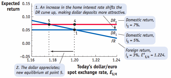 cases, the shocks make dollar deposits more attractive than euro deposits, but for different reasons. The shocks all lead to dollar appreciations.
- A Change in the Domestic Interest Rate
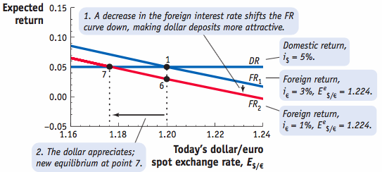 If rises by value , then, the domestic returns curve will shift up at magnitude because it is a horizontal curve.
- A Change in the Foreign Interest Rate
If falls by value , then, the foreign returns curve will shift down by magnitude .
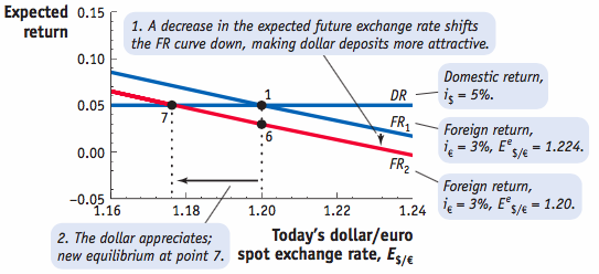 A Change in the Expected Future Exchange Rate
If falls by value , then, the foreign returns curve will shift down by magnitude .
Change in Domestic Interest Rate (if i$ rises):
- The domestic returns curve shifts up because higher domestic interest rates make dollar deposits more attractive.
- Traders prefer dollar deposits over euro deposits, to hold dollar deposits, traders need to sell euros and buy dollars, increasing the demand for dollars in the foreign exchange market
- Result: Increased demand for dollars relative to euros leads to an appreciation of the dollar and a decrease in the exchange rate (E) in terms of euros. This means it takes fewer dollars to buy one euro, indicating a stronger dollar.
Change in Foreign Interest Rate (If i€ falls):
The foreign returns curve shifts down because lower foreign interest rates make euro deposits less attractive. So Traders opt for dollar deposits over euro deposits. With thigher demand of dollars it increases and appreciates against euros which leads to selling euros and buying dollars.
Result: The home currency (dollar) appreciates, leading to a decrease in the exchange rate (E) in terms of euros.
Change in Expected Future Exchange Rate (E_($/€)^e falls):
A decrease in the expected future , In other words, they anticipate that in the future, it will take fewer dollars to buy one euro. When the expected future exchange rate decreases, it affects the returns investors expect to receive from investing in euros. The lower expected future exchange rate means that if investors hold euros now and exchange them for dollars in the future, they will receive fewer dollars than they previously expected. This lowers the expected returns from holding euros. As a result, the foreign returns curve shifts down because the expected returns from holding euros decrease.
With the decrease in expected returns from holding euros, dollar deposits become comparatively more appealing. Investors prefer assets denominated in dollars because they expect higher returns from them compared to holding euros. Therefore, investors start selling euros to buy dollars, increasing the demand for dollars in the foreign exchange market.
The increased demand for dollars and the selling pressure on euros cause the value of the dollar to appreciate relative to the euro. In other words, it takes fewer dollars to buy one euro.
This appreciation of the home currency (dollar) is represented by a decrease in the exchange rate (E), which shows how many dollars are needed to buy one euro. So, as E decreases, it means the dollar is strengthening against the euro.
15.2 Interest Rates in the Short Run: Money Market Equilibrium
The previous section laid out the essentials of the asset approach to exchange rates. The spot exchange rate is the output of this model, and the expected future exchange rate and the home and foreign interest rates are the inputs.
In this section, we discuss how the interest rates are determined in the short run.
Money Market Equilibrium in the Short Run: How Nominal Interest Rates Are Determined
Before going dep into the model, we must redefine our assumptions. Our long run assumptions were:
In the short run, the determination of nominal interest rates and money market equilibrium is influenced by various factors, including money supply, money demand, and nominal rigidities such as sticky prices. Let's break down the key points:
Money Market Equilibrium:In the short run, we focus on the supply of money provided by central banks (currency) and the demand for money from individuals and businesses.
- Equilibrium in the financial market occurs when the money supply (Ms) equals the money demand (Md), represented as Ms = Md.
Assumptions in the Short Run:
- Unlike the long run where prices (P) are flexible and adjust to market conditions to the market, . in the short run, prices are sticky or predetermined (P = P̅).
- Nominal interest rates (i) are fully flexible and adjust to bring the money market to equilibrium.
Nominal Rigidity:Nominal rigidity refers is the stickiness of prices, particularly nominal wages, which tend to be slow to adjust in the short run due to factors like long-term contracts.
- Sticky prices can lead to deviations from equilibrium in the short run, impacting the adjustment process of nominal interest rates.
Model Assumptions:
- These assumptions are made to account for the common characteristics of the short run, where nominal rigidities play a significant role in determining economic outcomes.
- Price stickiness and interest rate flexibility are key features of the short-run monetary model, allowing us to analyze how changes in money supply and demand affect nominal interest rates and overall market equilibrium.
In summary, the short-run monetary model considers sticky prices and flexible nominal interest rates to understand how money market equilibrium is achieved in the presence of nominal rigidities
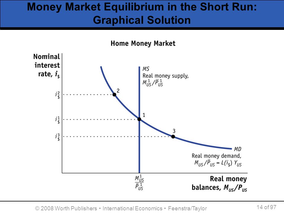
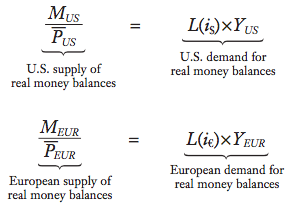 With those assumptions, we can rewrite our general monetary model as:
Adjustment to Money Market Equilibrium in the Short Run
The process of how the interest rate adjusts to bring the money market back to equilibrium in the short run. When the interest rate is higher than the equilibrium, meaning that real money demand is less than real money supply, there's an excess supply of money in the market
- Excess Supply of Money: At the higher interest rate, individuals and firms want to hold less money than what is available in the market. They seek to convert their excess money holdings into interest-bearing assets like bonds or savings accounts.
- Increased Savings and Lending: As people save more and seek to lend their excess money, borrowers notice an opportunity to borrow at lower costs. However, they will only borrow more if the cost of borrowing, i.e., the interest rate, falls.
- Competition among Lenders: To attract borrowers, lenders compete by offering lower interest rates. This competition drives down the interest rate.
- Equilibrium Restored: As the interest rate decreases, the demand for money increases while the excess supply decreases. Eventually, a new equilibrium is reached where the quantity of money demanded equals the quantity supplied, and the interest rate stabilizes at the equilibrium level.
Monetary Policy and Open Market Operations:
Central banks conduct monetary policy to stabilize economies by controlling the money supply. They often use open market operations (OMOs) to achieve this.
In OMOs, central banks buy or sell government bonds in the open market. When they buy bonds, they inject money into the economy, increasing the money supply. Conversely, when they sell bonds, they withdraw money from the economy, decreasing the money supply.
- An expansionary OMO, where bonds are bought, increases the money supply, leading to lower interest rates, injecting money into the economy and stimulation eco activity like spending & borrowing.
- a contractionary OMO, where bonds are sold, decreases the money supply, resulting in higher interest rates. This decreases liquidity, raises interest rates, and slows down borrowing and spending, thus cooling off an overheating economy or curbing inflation.
Bond prices & yields
In the bonds market it’s bond prices which are determined. In bond markets, interest rates are not directly determined but can be inferred from bond prices. Interest rate on return from bond.
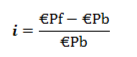
If one-year bonds promise to pay back €Pf (the final price) at the end of the year. If an investor purchases the bond today at a price of €Pb (the bond price), the final interest rate of return from holding that bond for one year can be calculated using the formula mentioned in the passage.
- EX: if €Pf is 100 (indicating that the bond will be redeemed at its face value) and €Pb is 95, the final interest rate will be 5.3% {(100-95)/95}. Similarly, if €Pf is 100 and €Pb is 90, the final interest rate will be 11.1%.
Bond prices and bond yields move inversely: as bond prices rise, yields fall, and vice versa.
Bond yield refers to the return an investor receives from holding a bond, expressed as a percentage of the bond's face value. It represents the interest income earned by the investor
Bond prices and yields move inversely because bond prices are determined by supply and demand dynamics in the bond market. When bond prices rise, it means investors are willing to pay more for the same fixed interest payment. As a result, the effective yield (or return) on the bond decreases.
Choosing Money or Interest Rates:
Central banks typically target interest rates rather than directly controlling the money supply. They set a target for the short-term interest rate and adjust the money supply to achieve that target.By targeting interest rates, central banks can influence borrowing, spending, and investment decisions, which are vital for economic growth and stability.
Adjusting the money supply to influence interest rates allows central banks to respond flexibly to changing economic conditions and financial market dynamics.
Short Run Money Market Equilibrium:
In the short run, assuming fixed price levels, the equilibrium interest rate is determined by the intersection of money supply and money demand in the money market.
Money supply is controlled by the central bank through OMOs, while money demand depends on factors like income, interest rates, and consumer preferences.
Changes in the money supply directly affect the nominal interest rate. An increase in the money supply lowers interest rates, while a decrease raises them, helping to stabilize the economy.
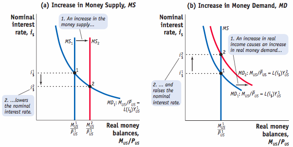 Effects of Changes in Money Supply and Real Income:
Increases in the money supply lower nominal interest rates by increasing the availability of funds for borrowing. Conversely, decreases in the money supply raise nominal interest rates by reducing the availability of funds.
Changes in real income, which represent changes in individuals' purchasing power, also influence nominal interest rates. Higher real income tends to increase borrowing and spending, leading to higher interest rates, while lower real income has the opposite effect.
The Monetary Model: The Short Run versus the Long Run
Expansion as a Permanent Policy: consider a situation in which a central bank decides to increase the money supply and let it grow at 5%. What are the implications of this particular money growth both in the short-run and in the long-run?
Short Run: When the central bank increases the money supply by 5% as a permanent policy, it leads to an immediate excess supply of money in the economy. However, because prices are sticky in the short run (meaning they don't adjust immediately to S+D), ppl & businesses find themselves holding more money than they desire given the prevailing interest rate. As a result, they seek to lend out or spend this excess money to earn returns or buys g&s . The increased demand for borrowing and spending, combined with the excess money supply, puts downward pressure on interest rates. Lenders, faced with increased demand for loans, may lower interest rates to attract borrowers. Additionally, lower interest rates make borrowing cheaper and more attractive, further stimulating demand for loans and spending. Lower interest rates incentivize borrowing and investment, leading to increased economic activity. However, excess liquidity and lower interest rates can also lead to a weaker currency. Investors seeking higher returns may move their funds to other countries or assets with higher interest rates, causing a depreciation of the domestic currency relative to others.
Long Run: In the long run, prices become more flexible and responsive to changes in supply and demand. As the excess money injected into the economy by the central bank persists, prices begin to increase to reflect this increased money supply and inflation sets in. The quantitative theory of money suggests that a 5% increase in the money supply leads to a 5% increase in inflation. As prices rise due to inflation, the real purchasing power of money decreases. This means that each unit of currency can buy fewer goods and services than before. In response to higher inflation and the decrease in the real value of money, nominal interest rates increase. The Fisher effect suggests that nominal interest rates adjust one-for-one with changes in expected inflation, thereby maintaining the real interest rate (the nominal rate minus the inflation rate). Higher nominal interest rates make borrowing more expensive and less attractive for businesses and consumers. As a result, investment and borrowing activity slow down in the economy. But they attract foreign investment , this increased demand for the domestic currency to invest in assets denominated in that currency leads to an appreciation of the currency, making it stronger relative to other currencies.
Expansion as a Temporary Policy:
- Short Run: If the increase in the money supply is perceived as temporary, it still leads to an initial excess supply of money in the economy. This excess liquidity drives down interest rates in the short run, similar to the permanent policy scenario. However, since expectations regarding future inflation and money supply growth remain unchanged, the impact on interest rates is temporary.
- Long Run: If the temporary policy becomes permanent, expectations regarding future inflation and money supply growth will eventually adjust. As prices become more flexible in the long run, the increase in the money supply will lead to higher inflation and, consequently, higher nominal interest rates. This leads to a stronger currency over the long term.
In summary, the short-run and long-run implications of monetary expansion differ due to the timing of price adjustments and the effect on expectations. In the short run, expansionary monetary policy leads to lower interest rates and a weaker currency, while in the long run, it leads to higher interest rates and a stronger currency as prices adjust to reflect the increase in the money supply.
Top of Form
Bottom of Form
15.3 The Asset Approach: Applications and Evidence
In the asset approach, we analyze the exchange rate between two currencies by considering the money supply and demand in one country along with the expected depreciation. Here's a breakdown of how it works:
- U.S. Money Market (Panel a):
- Money supply (Ms) is vertical because the interest rate (i) doesn't affect it.
- Money demand (Md) is downward sloping because as interest rates increase, demand falls.
- Equilibrium in the U.S. money market determines the interest rate.
- Foreign Exchange (FX) Market (Panel b):
- Domestic return (DR) is horizontal because the interest rate (i) is fixed.
- Foreign return (FR) is downward sloping because as the exchange rate (E) increases, interest rates fall.
- Equilibrium in the FX market is where uncovered interest parity (UIP) holds.
For the asset approach to work, UIP must hold, and there must be no capital controls, allowing free movement of capital.
Short-Run Policy Analysis:
- Temporary Shock to Home Money Supply:
- Increase in U.S. money supply raises M/P.
- Nominal interest rate (i) falls to counterbalance the initial effect.
- Lower DR and FR lead to a higher exchange rate (dollar depreciates).
- Temporary Shock to Foreign Money Supply:
- Foreign money supply expansion leads to a lower foreign interest rate (i).
- Decreased FR shifts the FX curve down, causing the dollar to appreciate.
Asset Approach Application:
- A temporary increase in home money supply lowers interest rates, leading to a higher exchange rate.
- A temporary change in foreign return shifts the FX curve, altering the exchange rate without changing the home country's interest rate.
The asset approach will be the joining of the money supply model and the FX diagram because, when you determine the interest rate with the money supply model, you can then use that interest rate to find the spot rate at its equilibrium:
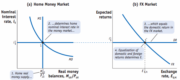
Thus, we can deduce some things:
- A temporary growth in the home money supply leads to a lower interest rate. This fall in the interest rate leads to a decrease in the domestic return in the FX market, leading to a higher exchange rate.
- If there is a temporary change in the foreign return on the FX market, then, only the FX curve will move and lead to a different exchange rate without changing the interest rate of the home country.
15.4 A Complete Theory: Unifying the Monetary and Asset Approaches
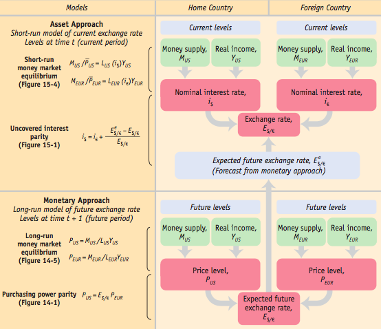 In this section, we extend our analysis from the short run to the long run and examine both temporary and permanent shocks. To do so, we need both the asset approach and the monetary approach.
Long Run Policy Analysis
We saw how temporary shocks in the short run did not affect long-run expectations. That is because these policies are temporary, but what if those policies are not? When a monetary policy shock is permanent, the long run expectation of the level of the exchange rate has to adjust, leading to the exchange rate predictions of the short run model to differ from those made when the policy shock was temporary.
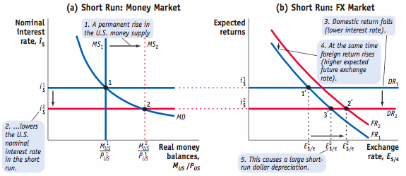 This observation leads to a very important conclusion: we cannot approach such analysis chronologically. We must understand the long run before being able to understand the short run effects.
Let’s look at the short-run and long-run effects of a permanent increase in money supply.
 In the long run, the increase in the money supply causes an increase in the price level by the same proportion so that the real money supply as well as the nominal interest rate are unchanged. In the forex market, the domestic return is unchanged because the interest rate is unchanged. However, the exchange rate rises because of the increase in the price level. Therefore, FR shifts up.
In the short run, there is a change in expectations, so the forex market is affected immediately. The expected exchange rate is higher, so FR shifts up. The dollar is expected to depreciate in the future, euros are more attractive today. In the short run, prices are sticky so the real money supply shifts right. The home interest rate falls. In the forex market, DR shifts down. The exchange rate depreciates even more.
In the short run, a permanent shock causes the exchange rate to depreciate more than it would under a temporary shock and more than it will end up depreciating in long run. |
E.g. Suppose that, all else equal, the home money supply permanently increases by 5% today, prices are sticky in the short run, so the domestic interest rate goes down from 6% to 2%; prices will fully adjust in one year’s time to today’s monetary expansion and PPP will hold again.
In the long run, a 5% increase in M means a 5% increase in P that will be achieved in one year. This implies a 5% rise in E. Finally, in the short run, to compensate investors for the 4% decrease in the domestic interest rate, arbitrage in the forex market requires that the value of the home currency be expected to appreciate at 4% per year; i.e., E must fall 4% in the year ahead. However, if E has to fall 4% in the next year and still end up 5% above its level at the start of today, then it must jump up 9% today: it overshoots its long-run level.
Overshooting
As we have observed, the temporary expansion of money supply has a much smaller effect than the permanent shock in the short run. Because, in the short run, the interest rate and exchange rate effects combine to create and instantaneous double effect as the price level does not change. We call that special phenomenon overshooting.
Here are usually how we can see the effects of overshooting:
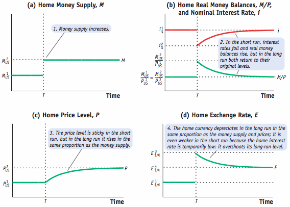 Nominal money supply is subject to a one-time increase.
- Real money balance rises instantaneously but comes back to its initial level in the long run, so does the nominal interest rate.
- Prices level is sticky in the short run but rises to a higher level in the long run, increasing in the same proportion as the nominal money supply.
- The exchange rate depreciates (rises) to a higher level in the long run. In the short run, the exchange rate rises even more, overshooting its long run level, then gradually decreasing over time.
This observation shows an even higher volatility in the exchange rates, proving the importance of a long-run nominal anchor.
15.5 Fixed Exchange Rates and the Trilemma
In this section, we adapt our existing theory to fixed exchange rates.
What is a Fixed Exchange Rate Regime?
Here, we set aside intermediate regimes and regimes that include capital controls. Instead, we focus on the case of a fixed rate regime without controls so that capital is mobile, and arbitrage is free to operate in the foreign exchange market.
Here the government itself becomes an actor in the forex market and uses intervention in the market to in influence the market rate. Exchange rate intervention takes the form of the central bank buying and selling foreign currency at a fixed price, thus holding the market exchange rate at a fixed level denoted.
In the long run, fixing the exchange rate is one kind of nominal anchor. What we now show is that a country with a fixed exchange rate faces monetary policy constraints not just in the long run but also in the short run.
Pegging Sacrifices Monetary Policy Autonomy in the Short Run: Example
Under a peg, the expected rate of depreciation is zero. Our short-run theory still applies, but with a different chain of causality.
Arbitrage is the key force. If the Danish central bank tried to supply more krone and lower interest rates, they would be foiled by arbitrage. Danes would want to sell krone deposits and buy higher-yield euro deposits, applying downward pressure on the krone. To maintain the peg, whatever krone the Danish central bank had tried to pump into circulation, it would promptly have to buy them back in the foreign exchange market.
- Under a float, the home monetary authorities pick the money supply M. In the short run, the choice of M determines the interest rate i in the money market; in turn, via UIP, the level of i determines the exchange rate E. The money supply is an input in the model
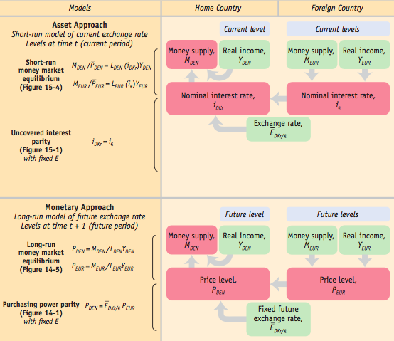 (an exogenous variable), and the exchange rate is an output of the model (an endogenous variable).
 - Under a fix, this logic is reversed. Home monetary authorities pick the fixed level of the exchange rate E. In the short run, a fixed E pins down the home interest rate i via UIP, forcing it to equal to foreign rate; in turn, the level of i determines the level of the money supply M necessary to meet money demand. The exchange rate is an input in the model (an exogenous variable), and the money supply is an output of the model (an endogenous variable).
Pegging Sacrifices Monetary Policy Autonomy in the Long Run: Example
Under a fix, home monetary authorities pick the fixed E. In the long run, the choice of E determines the price level P because of the PPP and the interest rate i via UIP. These, in turn, will determine the money supply M.
The Trilemma
Not all desirable policy goals can be simultaneously met. This representation is known as the trilemma because the 3 equations cannot hold at the same time, thus, we can only choose two because all 3 are incompatible.
- Fixed Exchange Rate
- May be desired as a means to promote stability in trade and investment.
- Represented here by zero expected depreciation.
- International Capital Mobility
- May be desired as a means to promote integration, efficiency, and risk sharing.
- Represented here by UIP, which results from arbitrage.
- Monetary Policy Autonomy
- May be desired a means to manage the home economy’s business cycle.
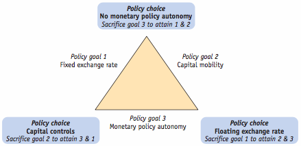 Represented here by the ability to set the home interest rate independently of the foreign one.
Chapter 16 – National and International Accounts: Income, Wealth, and the Balance of Payments
16.1 Measuring Macroeconomic Activity: An Overview
To understand how an open economy works, we must first know how a closed economy works. In a closed economy, economic activity is measured and recorded in the national income and product accounts. In an open economy, the additional flows are registered in a nation’s balance of payments accounts.
The Flow of Payments in a Closed Economy: Introducing the National Income and Product Accounts
We can define the cash flows in our economy as this:
- Gross National Expenditure
GNE represents the total expenditure on final foods and services by home consumers, businesses and government. It is defined as:
- Gross Domestic Product
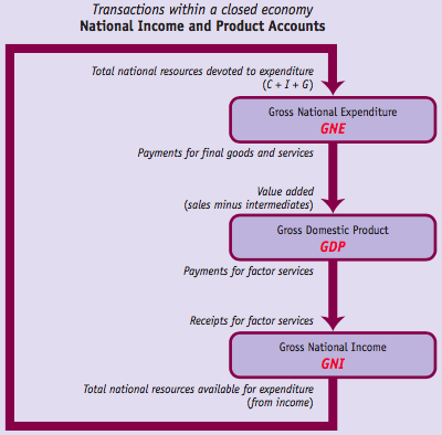 GDP represents the value of all goods and services produced as outputs by firms minus the value of all intermediate goods purchased as inputs by firms. In a closed economy, because intermediate goods produced and purchased cancel each other, we only have the final goods. Thus, on a closed economy:
- Gross National Income
GNI represents the total income resources of the economy. Thus, in our closed economy, we have GNE = GDP which is then paid as income to the factors of production in the form of GNI.
After this final step, income will be spent by consumers, forming the GNE. Thus, we can deduce that, in a closed market, GNE = GDP = GNI and so on. Expenditure is the same as product, which is the same as income.
The Flow of Payments in an Open Economy: Incorporating the Balance of Payments Accounts
Because the model for an open economy gets much more complex than the one with a closed one, we illustrate the cash flows with the figure bellow.
- Trade Balance (TB):
- Represents the difference between exports and imports of goods and services.
- When exports exceed imports, there's a trade surplus; when imports exceed exports, there's a trade deficit.
- Net Factor Income from Abroad (NFIA):
- Reflects the difference between payments received for factors of production (like capital, labor, and land) owned by domestic entities abroad and payments made to foreign entities for factors owned by them in the home country.
- Positive NFIA means the country earns more from its factors abroad than it pays to foreign factors at home.
- Net Unilateral Transfers (NUT):
- Accounts for non-tangible transfers (gifts) between countries, such as aid, remittances, and grants.
- Positive NUT implies the country receives more unilateral transfers than it gives out.
- Gross National Disposable Income (GNDI):
- It's the sum of Gross National Income (GNI) and Net Unilateral Transfers (NUT).
- Represents the total income available for spending or saving in the economy after accounting for unilateral transfers.
- Current Account (CA):
- Summarizes all international transactions in goods, services, income, and unilateral transfers.
- CA = Trade Balance (TB) + Net Factor Income from Abroad (NFIA) + Net Unilateral Transfers (NUT).
- Financial Account (FA):
- Captures the difference between assets exports and imports, reflecting the country's capacity to spend on assets like stocks, bonds, and real estate in other countries.
- Capital Account (KA):
- Measures the value of capital transfers received minus the capital transfers given, representing the transfer of assets between countries.
The part in green are all the cash flows reported in the nation’s balance of payments (BOP) accounts while the part in purple is the one we just discussed in the closed economy. In this representation of an open economy, there are five main points that we need to consider:
- As before, our model starts with the GNE, but in the case of an open economy, we must consider the fact that countries import and export goods and services for various reasons. To get the GDP, we subtract imports because those goods are not sold by domestic firms. Exports are added because those goods are sold by domestic firms. The difference between payments received for exports and payments made for imports is called the trade balance (TB = EX - IM) and it equals net payments to domestic firms due to trade.
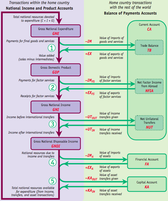
- Our second point is to consider factor service imports, which are domestic payments to capital, labour and land owned by foreign entities. As it is not paid at home, it is subtracted from income. The opposite goes for factor service exports which are foreign payments to capital, labour and land owned by domestic entities. The value of factor service exports minus factor service imports is called the net factor income from abroad (NFIA = EXFS – IMFS).
- At our third point, we see that home countries may not retain all of its earned income. Domestic entities could, for example, give aid or remittances for migrants to their families back home, and similarly they could receive gifts from aboard as well. These nonmarket transactions, or unilateral transfers, are considered in our model as net unilateral transfers (NUT), which is defined as the value of unilateral transfers received minus unilateral transfers given. Leading us to a new kind of cash flow known as the gross national disposable income (GNDI).
Note that the balance of payments considers the three things we just saw and reports their sum as the current account (CA), a tally of all international transactions in goods, services, and income that occur through market transactions or transfers.
- The fourth point we must make is that GNDI is not representative of a country’s capacity to spend. It may be increased or decreased by trading assets with other countries. The value of those assets exports minus the assets imports is called the financial account (FA).
- The final point we make is that a country may not only pay or sell assets, it may also give them or receive them as gifts. Such asset transfers are measured by capital account (KA), which is the value of capital transfers from the rest of the world minus those to the rest of the world.
This model leads us to one important conclusion: As we start with GNE, add in everything in the balance of payments accounts and still end up with the GNE, the sum of all the items in the balance of payments must be equal to 0.
16.2 Income, Product and Expenditure
Now that we learned about the concepts of an open economy, let’s use them to define the key accounting concepts in the two sets of accounts and put them to use.
Three Approaches to Measuring Economic Activity
There are three main approaches to the measure of aggregate economic activity of a country:
- The expenditure approach: looks at the demand for goods and is based on GNE.
- The product approach: looks at the supply for goods and is based on GDP.
- The income approach: focusses on payments to owners of factors and is based on GNI and GNDI.
From GNE to GDP: Accounting for Trade in Goods and Services
We know that GNE is calculated as:
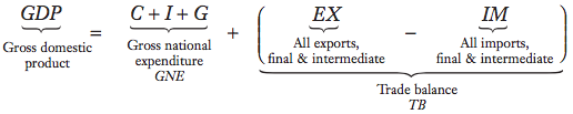 In an open economy, we also must consider the imports and the export of final and intermediate goods which will lead us to the GDP. We especially cannot forget about intermediate goods. Thus, we can say that:
Adding the trade balance, we can notice that it can be negative or positive:
- If TB > 0, exports are greater than imports and we can say that a country has a trade surplus.
- If TB < 0, imports are greater than exports and we can say that a country has a trade deficit.
From GDP to GNI: Accounting for Trade in Factor Services
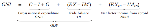 Now, that we found the formula for GDP, let’s allow our model to consider factor services such as income payments to foreign entities for factor services imported (IMFS) and income receipts for factor services exported by the home country (EXFS).
And once again, we can notice that the NFIA can be negative or positive for the same reasons as TB.
From GNI to GNDI: Accounting for Transfers in Income
Now, we consider those gifts some countries may receive that we discussed in (3). If a country receives transfers worth UTIN and gives transfers worth UTOUT, then, its net unilateral transfers can be defined as:
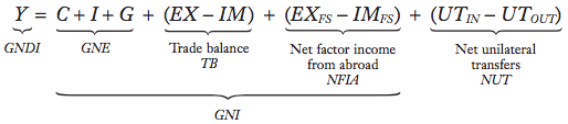 This new formula helps us to define the GNDI that we will now denote Y as it represents the disposable income a country can give. Thus, we obtain:
Note that on this formula, the sum of TB, NFIA and NUT is what we call the current account. We will then denote it CA in our equation for Y from now on.
What the Current Account Tells Us
The current account tells us is if a country is spending more or less than its income. The equation we have just seen that:
is the equation of the open economy called the national income identity. Thus, knowing this equation, we can deduct that:
- If GNDI > GNE, then CA > 0.
- If GNDI < GNE, then CA < 0.
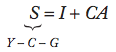 If we subtract C+G from both sides of that identity, we obtain a new one showing us the difference between national saving and investment:
This equation is called the current account identity, and knowing this equation we can deduct that:
- If S > I, then CA > 0.
- If S < I, then CA < 0.
16.3 The Balance of Payments
Here, we look at international transactions. They are important because they tell us how the current account is financed, and, hence, whether a country is becoming more or less indebted to the rest of the world.
Accounting for Asset Transactions: The Financial Account
We first look at the financial account. It measures all movements of assets across the international border and considers all kind of assets such as real assets, financial assets, or even assets owned by the government. We obtain the home economy’s net overall balance on asset transactions, known as the financial account by subtracting asset imports from asset exports:
Accounting for Asset Transactions: The Capital Account
Now, we look at the capital account. The capital account covers the remaining balance of payment accounts such as non-produced assets (copyrights, patents, etc..) or unilateral transfers (gifts of assets or forgiveness of debt). We obtain the home economy’s capital account by subtracting capital transfers received from capital transfers given:
As with unilateral income transfers, capital transfers must be accounted for properly. For example, the giver of an asset must deduct the value of the gift in the capital account to offset the export of the asset, which is recorded in the financial account, because in the case of a gift the export generates no associated payment. Similarly, recipients of capital transfers need to record them to offset the import of the asset recorded in the financial account.
Accounting for Home and Foreign Assets
We can separate the asset trades into two kinds of assets: the ones issued by the home entities (home assets) and the ones issued by foreign entities (foreign assets). From the home perspective, a foreign asset is a claim on a foreign country. This kind of asset is an external asset. Conversely, from the home perspective, a home asset is a claim on the home country. This kind of asset is an external liability.
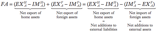 If we use superscripts H and F to denote home and foreign assets, we break down the financial accounts as the sum of the next exports of each type of asset:
Thus, financial assets are equal to the addition to external liabilities minus the additions to external assets.
How the Balance of Payments Work: A Macroeconomic View
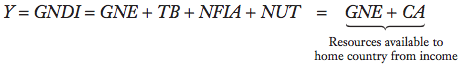 Summarizing everything we now know from the home market, we know that:
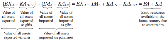 But that we should also consider the assets imported and exported:
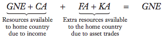 Adding the last two expressions, we arrive at the value of the total resources available to the home country for expenditure purposes, which must equal the GNE:
![]() We can cancel GNE on both sides of the equation leading us what we call the balance of payments (BOP) identity.
We can cancel GNE on both sides of the equation leading us what we call the balance of payments (BOP) identity.
How the Balance of Payments Work: A Microeconomic View
Another way of looking at the equation we just found is to look behind the three variables that compose it. We know that:
As we can observe from these equations, there are 12 transactions types and 3 accounts in which they appear. We define two types of transactions, the ones that make the accounts grow and the ones that make the accounts fall.
In the first case, we call those transactions BOP credit. There are six of them:
- Current account (CA):
- Exports of goods and services ()
- Exports of factor services ()
- Unilateral transfers received ()
- Financial account (FA):
- Exports of home and foreign assets (;)
- Capital account (KA)
- Capital transfers received ()
In the second case, we call those transactions BOP debit. There are six of them:
- Current account (CA):
- Imports of goods and services ()
- Imports of factor services ()
- Unilateral transfers given ()
- Financial account (FA):
- Imports of home and foreign assets (;)
- Capital account (KA)
- Capital transfers given ()
Those transactions lead to a principle allowing us to explain the BOP in an easy way:
If a party A engages a transaction with a counterparty B, then A receives from B an item of value, and in return, B receives from A an item of equal value.
In real life, the BOP accounts will not be equal to 0 because statistical agencies will never be able to track every single international transaction correctly. But if we look at one account, we can define a country in a special way. If a country has a current account surplus, then it is called a (net) lender while if it has a current account deficit, the country is called a (net) borrower.
16.4 External Wealth
Economic variables are not the only things we are interested in. We also care about what a country is worth in terms of wealth. Therefore, we calculate a home country’s ‘net worth’ or external wealth (W) with respect to the rest of the world (ROW) to analyse it.
The Level of External Wealth
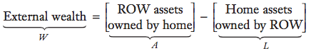 We define the external wealth as the value of total external assets (A) minus the value of total external liabilities (L). Thus, we obtain:
A country’s level of external wealth is also called its net international investment position or net foreign assets. We can define two states:
- W > 0, the home country is a net creditor country: external assets exceed external liabilities; thus, the country owes less to the ROW than the ROW owes to the country.
- W < 0, the home country is a net debtor country: external liabilities exceed external assets; thus, the country owes more to the ROW than the ROW owes to the country.
Of course, there is more in the wealth of a country than its external wealth but, as we focus on international relations, we will only focus on external wealth.
Changes in External Wealth
There are two main reasons why a country’s level of external wealth changes over time:
- Financial flows: net exports of foreign assets cause an equal decrease in the level of external assets, leading to a decrease in external wealth and the opposite also holds.
- Valuation effects: the value of existing external assets and liabilities may change over times because of capital gain or losses like price level effects or exchange rate effects.
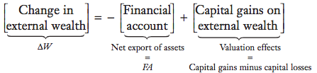
Thus, we can say that:
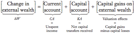 Recalling the BOP identity: the current account plus the capital account plus the financial account equal zero. We get:
Thus, this formula tells us that there are three ways a country can increase its external wealth:
- With a CA surplus (with a growth in its economy)
- With a KA surplus (with the charity of other countries)
- With positive capital gains (with the help of windfalls)
Over the long run, these changes in the external wealth will gradually accumulate.
Bottom of Form
Bottom of Form