AP Statistics: Ultimate Study Guide
(I need to add Sentence Stems, calculator steps, and )
General Strategies for AP Statistics
Be Specific:
Always include numerical values and context.
Example: Instead of saying "a large number of students," specify "25 out of 100 students." This clarifies the scale and ensures a precise understanding.
Define and Show Work:
Clearly define variables and show all calculations step-by-step. This not only demonstrates your understanding but can also earn partial credit for correct methods, even if the final answer is wrong.
Example: If X is the number of successes in a binomial distribution, define it before starting your calculation.
Read Carefully:
Understand the question requirements before answering. Highlight key points or terms to focus your response.
Check Your Answers:
After solving, review your solution. Ensure it fits the problem context and check for calculation errors.
Descriptive Statistics
CUSS Method (for describing distributions):
Center: Use the mean or median depending on the data's skewness.
Example: The median is better for skewed data, while the mean is appropriate for symmetrical data.
Unusual Features: Identify outliers or gaps and discuss their impact.
Example: An outlier might significantly affect the mean but have little effect on the median.
Spread: Discuss variability using range, interquartile range (IQR), or standard deviation.
Example: Standard deviation measures how spread out the data is from the mean.
Shape: Describe the distribution's shape:
Symmetrical: Mean ≈ Median.
Skewed Right: Tail on the right; mean > median.
Skewed Left: Tail on the left; mean < median.
Unimodal: One peak in the data
Bimodal: Two peaks in the data.
Example Scenario:
For a histogram of test scores:
Center: Mean = 75.
Spread: Standard deviation = 10.
Shape: Skewed right, indicating more low scores.
SOCS Method (for analyzing data sets and graphs)
Shape: Identify overall pattern and shape of the data distribution.
Example: Symmetrical, skewed left/right, or unimodal/bimodal.
Outliers: Detect any points that fall far outside the general pattern.
Example: In a dataset with test scores, a score of 100 might be an outlier if most scores are between 50 and 70.
Center: Determine the typical value, using mean or median.
Example: Median is better when there are outliers.
Spread: Measure variability using range, IQR, or standard deviation.
Example: An IQR of 20 indicates that the middle 50% of data points are spread across 20 units.
DUFS Method (for describing scatterplots)
Direction: Determine if the relationship is positive, negative, or neither.
Example: A positive direction means that as x increases, y increases.
Unusual Features: Look for outliers or clusters that do not fit the general pattern.
Example: A point far from the rest of the data in a scatterplot of height vs. weight.
Form: Identify the form of the relationship (linear or nonlinear).
Example: A linear form suggests a straight-line relationship, while a curved pattern indicates nonlinearity.
Strength: Assess how tightly the points follow the form.
Example: A strong correlation means points closely follow a line.
Describing a Relationship (STD)
Strength: Strong, moderate, or weak.
Example: r=0.9 suggests a strong linear relationship.
Trend: Identify if the relationship is linear or nonlinear.
Example: A curved scatterplot indicates a nonlinear trend.
Direction: Positive or negative.
Example: A positive correlation means that as one variable increases, so does the other.
Probability Distributions
Binomial Distribution: (BINS)
B: Binary-either success or failure
I: Independent trials
N: Number of trials fixed
S: Success probability stays the same
Properties: Fixed number of trials (n), binary outcomes (success/failure), independent trials, and constant probability of success (p).
Formula:
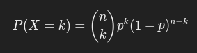
Where

is the number of ways to choose k successes from n trials.
Example: The probability of flipping exactly 3 heads in 5 coin tosses.
Geometric Distribution: (BITS)
B: Binary-either success or failure
I: Independent trials
T: Trials until success
S: Success probability stays the same
Properties: Trials continue until the first success, with constant probability p.
Formula:
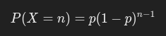
Example: Probability of rolling a six on the third dice roll.
Inferential Statistics
Constructing Confidence Intervals (PANIC method):
P: Define the parameter of interest (mean μ\muμ or proportion ppp).
A: State assumptions:
Random Sample
Normality: For means, use CLT if n≥30; for proportions, check np≥10 and n(1−p)≥10.
N: Name the interval (e.g., 1-proportion z-interval).
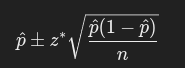
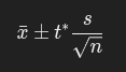
I: Calculate the interval:
For proportions:
For means (unknown σ):
C: Conclude in context (e.g., "We are 95% confident that the true proportion is between...").
Hypothesis Testing (PHANTOMS method):
P: Define the parameter and significance level (α).
H: State hypotheses (H0 and Ha).
A: Check assumptions (randomness, normality, independence).
N: Identify the test (e.g., 1-proportion z-test).
T: Calculate the test statistic:
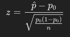
For proportions:
O: Find the p-value.
M: Make a decision (p<α: Reject H0).
S: State the conclusion in context.
Regression Analysis
Slope Interpretation: For each unit increase in x, y changes by the slope value.
Example: If the slope is 2.5, the predicted score increases by 2.5 points for each additional hour studied.
Coefficient of Determination (R2):
Indicates the percentage of variability in y explained by x.
Example: R2= 0.75 means 75% of the variation in test scores is explained by study hours.
Residual Plots:
No pattern suggests a good linear fit.
Curves or patterns suggest a nonlinear relationship or the need for transformation.
Experimental Design
Sampling Methods:
Simple Random Sample (SRS): Equal chance for all samples.
Stratified (Random): Divide into strata, then sample from each.
Cluster: Randomly select clusters and sample all within them.
Systematic: Sample every kth individual after a random start.
Voluntary: Sample is selected in a way that people do not have to respond
Convenience: Sample people who are easy or comfortable to collect information from.
Bias Types:
Voluntary Response Bias: Participants self-select; often not representative.
Undercoverage: Some groups excluded from the sample.
Non-response Bias: Selected individuals do not respond.
Response Bias: Misleading or biased questions lead to incorrect responses.
Wording of Questions: Question is worded so that a certain response is given.
Key Formulas and Concepts
Standard Deviation (σ or s):
Measures data spread from the mean.Z-Score:
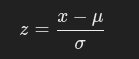
Indicates how many standard deviations x is from the mean.
Central Limit Theorem (CLT):
For large n, the sampling distribution of the mean is approximately normal.
Types of Errors in Hypothesis Testing
Type I Error (α): Rejecting H0 when it’s actually true.
Type II Error (β): Failing to reject H0 when Ha is true.
Power of a Test:
Probability of correctly rejecting H0; increasing sample size improves power.
Types of Graphs
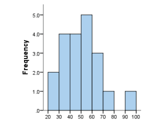
1. Histogram
Description: Displays the frequency distribution of numerical data by grouping data into intervals (bins).
Usage: Useful for identifying the shape of a distribution (e.g., symmetrical, skewed).
Example: Showing the distribution of test scores among students.
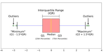
2. Boxplot (Box-and-Whisker Plot)
Description: Visual representation of the 5-number summary (minimum, Q1, median, Q3, maximum).
Usage: Ideal for identifying outliers and comparing distributions.
Example: Comparing the spread of scores between two classes.
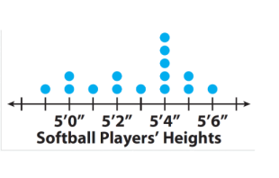
3. Dotplot
Description: Displays individual data points on a number line.
Usage: Useful for small datasets to show frequency and distribution.
Example: Representing the number of pets owned by students in a class.
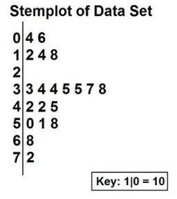
4. Stemplot (Stem-and-Leaf Plot)
Description: Splits data into stems (the leading digits) and leaves (the trailing digits).
Usage: Preserves raw data while showing distribution.
Example: Displaying exam scores (e.g., 85 → stem: 8, leaf: 5).
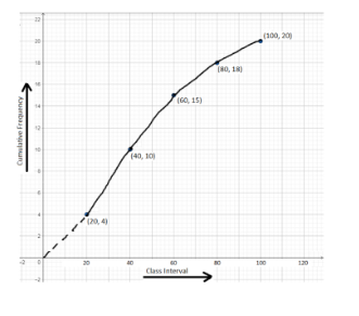
5. Ogive (Cumulative Frequency Graph)
Description: Plots cumulative frequencies, showing the number of observations below each value.
Usage: Helpful for understanding percentiles and cumulative data.
Example: Showing the cumulative percentage of students scoring below certain thresholds on a test.
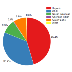
6. Pie Chart
Description: A circular chart divided into sectors representing proportions.
Usage: Best for categorical data and displaying relative frequencies as percentages.
Example: Visualizing the proportion of students choosing different subjects.
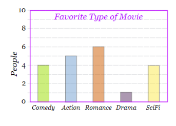
7. Bar Graph
Description: Uses bars to represent frequencies of categorical data.
Usage: Useful for comparing categories.
Example: Comparing the number of students in different grade levels.
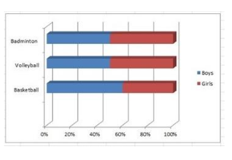
8. Segmented Bar Graph
Description: A bar graph divided into segments, each representing a category within a whole.
Usage: Useful for comparing the composition of different groups.
Example: Showing the distribution of favorite sports across different grades.
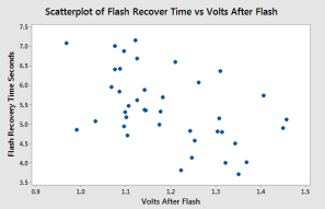
9. Scatterplot
Description: Plots pairs of quantitative data points on a coordinate plane.
Usage: Shows relationships between two variables (correlation, trends, outliers).
Example: Examining the relationship between study hours and exam scores.
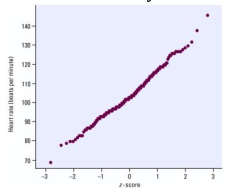
10. Normal Probability Plot
Description: Plots data points against a normal distribution to assess normality.
Usage: Determines if data is approximately normally distributed.
Example: Checking if the heights of students follow a normal distribution.
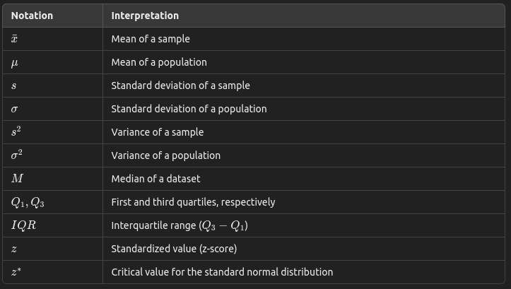
List of Notations and Interpretations
1. Descriptive Statistics Notations
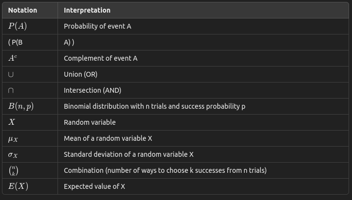
2. Probability Notations
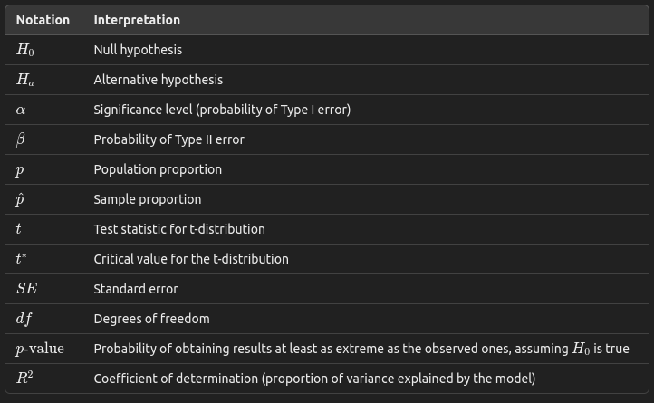
3. Inferential Statistics Notations
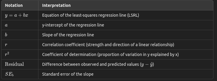
4. Regression and Correlation Notations
5. Distribution and Sampling Notations
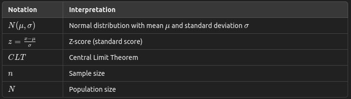
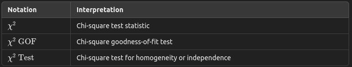
6. Chi-Square Notations
Ultimate Interpretations Guide
Unit 1: Exploring One-Variable Data
Standard Deviation: The context typically varies by SD from the mean of mean.
Example: The height of power forwards in the NBA typically varies by 1.51 inches from the mean of 80.1 inches.
Percentile: Percentile % of context are less than or equal to value.
Example: 75% of high school student SAT scores are less than or equal to 1200
Z-score: Specific value with context is z-score standard deviations above/below the mean.
Example: A quiz score of 71 is 1.43 standard deviations below the mean. (z = -1.43)
Describe a distribution: Be sure to address shape, center, variability and outliers. (in context)
Example: The distribution of student height is unimodal and roughly symmetric. The mean height is 65.3 inches with a standard deviation of 8.2 inches. There is potential upper outlier at 79 inches and a gap between 60 and 62 inches.
Unit 2: Exploring Two-Variable Data
Correlation: The linear association between x-context and y-context is weak/moderate.strong (strength) and positive/negative (direction).
Example: The linear association between student absences and final grades is fairly strong and negative. (r = -0.93)
Residual: The actual y-context was residual above/below the predicted value when x-context = #.
Example: The actual heart rate was 4.5 beats per minute above the number predicted when Matt ran for 5 minutes.
y-intercept: The predicted y-context when x = 0 context is y-intercept.
Example: The predicted time to checkout at the grocery store when there are 0 customers in
line is 72.95 seconds.
Slope: The predicted y-context increases/decreases by slope for each additional x-context.
Example: The predicted heart rate increases by 4.3 beats per minute for each additional
minute jogged.
Standard Deviation of Residuals (s): The actual y-context is typically about s away from the value predicted by the LSRL.
Example: The actual SAT score is typically about 14.3 points away from the value predicted
by the LSRL.
Coefficient of Determination (r²): About r²% of the variation in y-context can be explained by the linear relationship with x-context.
Example: About 87.3% of variation in electricity production is explained by the linear relationship with wind speed.
Describe the relationship: Be sure to address strength, direction, form and unusual features (in context)
Example: The scatter plot reveals a moderately strong, positie, linear association between the weight and length of rattlesnakes. The point at (24.1, 35.7) is potential outlier
Unit 4: Probability, Random Variable and Probability Distributions
Probability P(A): After many many context the proportion of times that context A will occur is about P(A)
Example: P(heads) = 0.5
After many many coin flips the proportion of times that heads will occur is about 0.5.
Conditional Probability P(A|B): Given context B there is a P(A|B) probability of context A.
Example: P(red car | pulled over) = 0.48.
Given that a car is pulled over, there is a 0.48 probability of the car being red.
Expected Value (Mean): if the random process of context is repeated for a very large number of times, the average number of x-context we can expect is expected value. (decimals are okay)
If the random process of asking a student how many movies they watched this week is repeated for a very large number of times, the average number of movies we can expect is 3.23 movies.
Binomial Mean: After many many trials the average # of success context out of n is mean.
Example: AFter many many trials the average number of property crimes that go unresolved out of 100 is 80.
Binomial Standard Deviation: The number of succes context out of n typically varies by standard deviation from the mean of mean.
Example: The number of property crimes that go unsolved out of 100 typically varies by 1.6 crimes from the mean of 80 crimes.
Unit 5: Sampling Distributions
Standard Deviation of Sample Proportions: The sample proportion of success context typically varies by standard deviation from the true proportion of p.
Example: The sample proportion of students that did their AP stats homework last night typically varies by 0,12 from the true proportion of 0.73.
Standard Deviation of Sample Means: The sample mean amount of x-context typically varies by standard deviation from the true mean of mean.
Example: The sample mean amount of defective parts typically varies by 5.6 parts from the true mean of 23.2 parts.
Unit 6, 7, 8 & 9: Inference for Proportions, Means, and Slope
Confidence Interval (A, B): We are % confident that the interval from A to B captures the true parameter context.
Example: We are 95% confident that the interval from 0.23 to 0.27 captures the true proportion of flowers that will be red after cross-fertilizing red and white.
Confidence Level: If we take many many samples of the same size and calculate a confidence interval for each, about confidence level % of them will capture the true parameter in context.
Example: If we take many, many samples of size 20 and calculate a confidence interval for each, about 90% of them will capture the true mean weight of a soda case.
P-Value: Assuming Ho in context, there is a p-value probability of getting the observed result or less/great/more extreme, by chance.
Assuming the mean body temperature is 98.6 °F, there is a 0.023 probability of getting a sample mean of 97.9 °F or less, purely by
chance.
Conclusion for a Significance Test: Because of p-value of p-value < / > α we reject / fail to reject Ho. We do / do not have convincing evidence for Ha in context.
Example: Because the p-value 0.023 < 0.05, we reject H0. We do have convincing evidence that the mean body temperature is less than 98.6 °F.
Type I Error: The Ho context is true, but we find convincing evidence for the context.
Example: The mean body temperature is actually 98.6 °F, but we find convincing evidence that the mean body temperature is less than 98.6 °F.
Type II Error: The Ha context is true, but we don’t find convincing evidence for the context.
Example: The mean body temperature is actually less than 98.6 °F, but we don’t find convincing evidence that the mean body temperature is less than 98.6 °F.
Power: If Ha context is true at a specific value, there is a power probability the significance test will correctly reject Ha
Example: If the true mean body temperature is 97.5 °F, there is a 0.73 probability the significance test will correctly reject 98.6
Standard Error of the Slope : The slope of the sample LSRL for x-context and y-context typically varies from the slope of the population LSRL by about SE.
Example: The slope of the sample LSRL for absences and final grades typically varies from the slope of the population LSRL by about 1.2 points/absence.