Ultimate AP Pre Calc Notes
Ch. 1 - The Basics
Point-Slope Form:
(y - y1) = m(x - x1)
Quadratic Formula:
x = (-b ± √(b2 - 4ac)) / (2a)
Average Rate of Change:
m = (f(b) - f(a)) / (b - a)
Difference Quotient:
(f(x + h) - f(x)) / h
Vertical Line Test → f(x) is not a function if the vertical line intercepts with more than one point
Perpendicular lines have negative reciprocals
Transformations | |
|---|---|
Linear | y = a(x -h) + k |
Quadratic | y = a(x - h)² + k |
Cubic | y = a(x - h)³ + k |
Square Root | y = a√(x - h) + k y = a(x - h)1/2 + k |
Reciprocal | y = a(1 / (x - h)) + k |
Exponential | y= ab(x - h) + k |
Combinations of Functions | |
|---|---|
Sum | (f+g)(x) = f(x) + g(x) |
Difference | (f-g)(x) = f(x) - g(x) |
Product | (fg)(x) = f(x) * g(x) |
Quotient | (f / g)(x) = f(x) / g(x), g(x) ≠ 0 |
Composite | f(g(x)) |
**The domain of a composite function is restricted by the domain of the input function
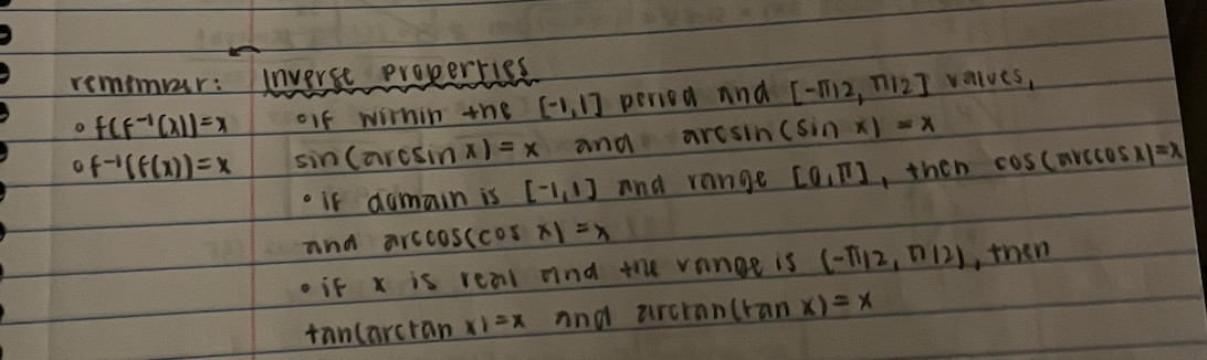
Inverse Functions
The composition of inverse functions is equal to 0 → f(f-1(x))=x
To find inverse functions, replace f(x), or y, with the x-variable and x with a y- . Then, solve for y, or f-1(x).
Scatterplots
The sum of the square of differences between the actual values and the model values is called the sum of the squared differences.
The model that has the least sum is called the least squared regression line for the data.
Residual: (e) the difference between the actual value and the value predicted by the model
e = y - ŷ (Actual - Predicted)
Correlation coefficient: (r) how close the best fit is to the the points
Calculator: Stat → Edit → Stat → 2nd Menu → Linreg
Finding Types of Functions (Linear, Quadratic, Exponential, Neither)
Using the given table, find AROC, the 2nd Difference, and Ratio
All AROC are Equal → Linear
All 2nd Difference are Equal → Quadratic
All Ratios are Equal → Exponential
Concave up → AROC over equal length input value intervals is increasing
Concave down → AROC over equal length input value intervals is decreasing
Ch 2 - Polynomials & Rational Functions
Graph of polynomial functions are continuous (no breaks, holes, or gaps)
Extrema: the minimums and maximums of a function
Relative/Local Extrema
Absolute/Global Extrema
∅ = Empty set
Between two real zeros, there must be at least one local min or max
Even-degree polynomials have either a global min or global max
Point of Inflection: occurs where the function changes from concave up to concave down, or vice versa
ROC changes from increasing to decreasing
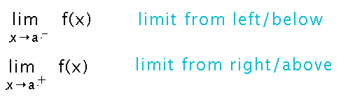
Limits
End Behavior: what happens to the values of f(x) as x increases or decreases without bounds
To find, use leading coefficient test (e.g. LC is odd/even, negative/positive)
Zeros of a Polynomial
x = a → zero/solution of polynomial
(x - a ) → factor of polynomial
(a, 0) → x-intercept of polynomial
Imaginary Numbers
i = √(-1)
Complex Number: a + bi
Complex Conjugate: a - bi
To rationalize imaginary numbers (in denominators), multiply by the conjugate
Division Algorithm Theorem: f(x) = d(x)*g(x) + r(x)
where f(x) is = dividend, d(x) = divisor, g(x) = quotient, and r(x) = remainder
Remainder Theorem: If polynomial f(x) is divided by x-h, then the remainder is r = f(k)
Factor Theorem: A polynomial f(x) has a factor (x-h) if and only if f(k) = 0
Rational Root Test: If a polynomial f(x) has integer coefficients, then every rational zero of f(x) has the form p / q
where p = factor of constant term and q = factor of leading coefficient
Rational Functions
f(x) = N(x) / D(x) = anxn / bmxm
VA(s) are zeros of the denominator, HA is determined by the degrees of N(x) and D(x)
n < m → y = 0
n = m → y = LC/LC
n > m → no HA (slant asymptote, if n < m by 1)
SA is found by dividing N(x) by D(x)
Graphing Rational Functions
Simplify f(x), if possible, and list all restrictions
Find and plot y-intercepts
Find and plot the zeros of the numerator
Find the VA (zeros of denominator)
Find and sketch other asymptotes with a dashed line
Plot min. 2 points between asymptotes and one point beyond each x-intercept and VA
Use smooth curves to complete graph
Ch. 3 - Exponentials and Logs
Log Form: y = loga x
a must be >1 and positive
x must be positive
Exponential Form: ay = x
Prop. of Logs | |
|---|---|
Product Property |
|
Quotient Property |
|
Power Property |
|
Change of Base Formula:
loga x = ln x / ln a
loga x = logb x / logb a
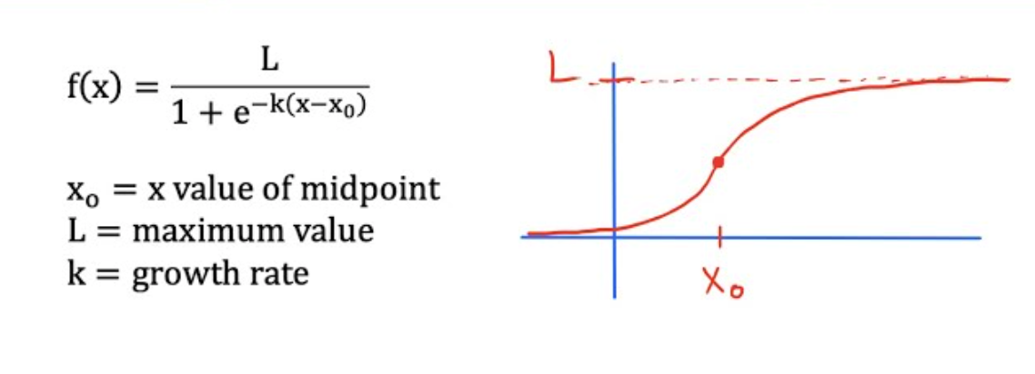
Logistic Model
Sequences | Prop. of Successive Terms | Formulas |
|---|---|---|
Arithmetic | Common difference |
|
Geometric | Common ratio |
|
Calculating Interest
Normal Interest: A = P(1 + (r / n))nt
Compound Interest: A = Pert
Ch. 4 - Trig Functions (radians)
Counter-clockwise (CCW) angle → +θ
Clockwise (CW) angle → -θ
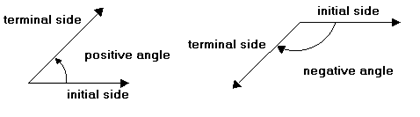
Coterminal Angles: angles which share the same terminal side in standard positon
There’s an infinite number of coterminal angles
Arc Length Formula: s = θr
Unit Conversion: π rad = 180°
Trigonometric Functions | Inverse Trig Functions | |
|---|---|---|
sin θ = y / r | csc θ = r / y | arcsin (y / r) = θ |
cos θ = x / r | sec θ = r / x | arccos (x / r) = θ |
tan θ = y / x | cot θ = x / y | arctan (y / x) = θ |
**Solve the right triangle → find all angles and sides
**Remember to add 2π, n∈ℤ if there’s no restricted range
The Unit Circle

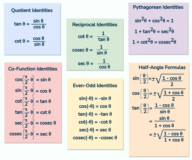
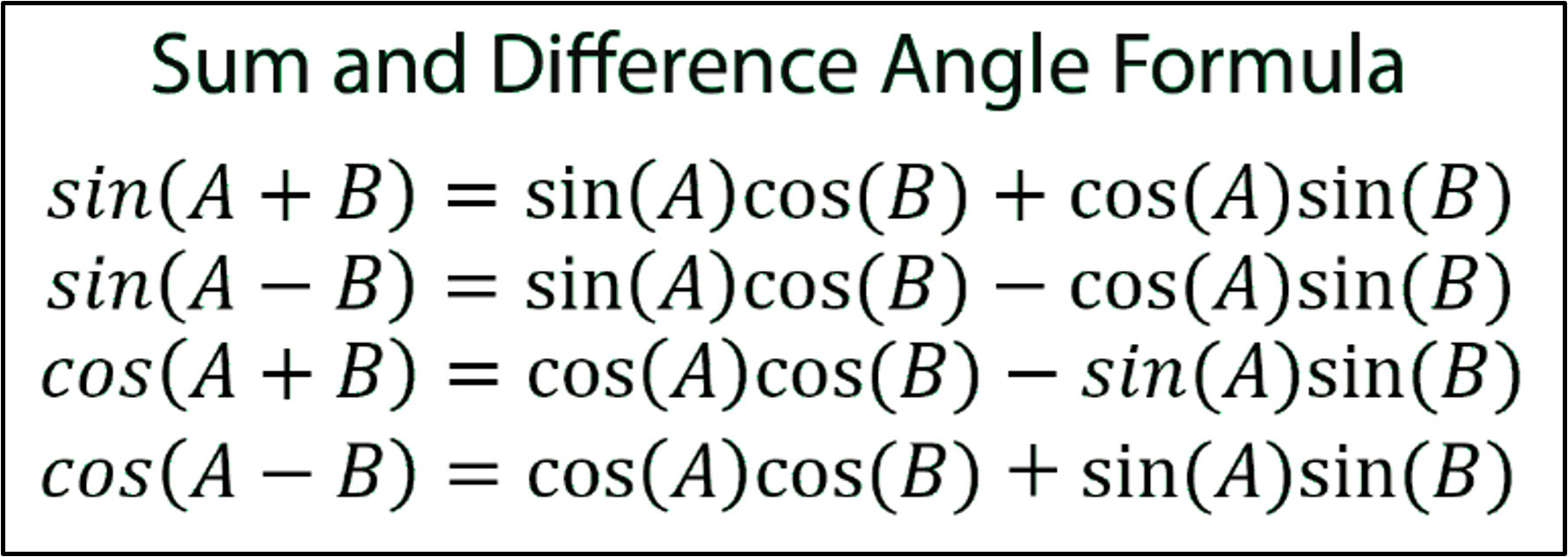
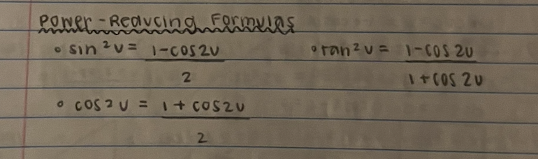
Trig Identities/Formulas
All Students Take Calculus: Mnemonic to remember in which quadrants the trig functions are positive

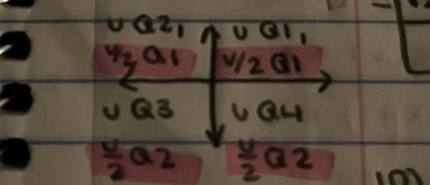
Half-Angle Quadrants
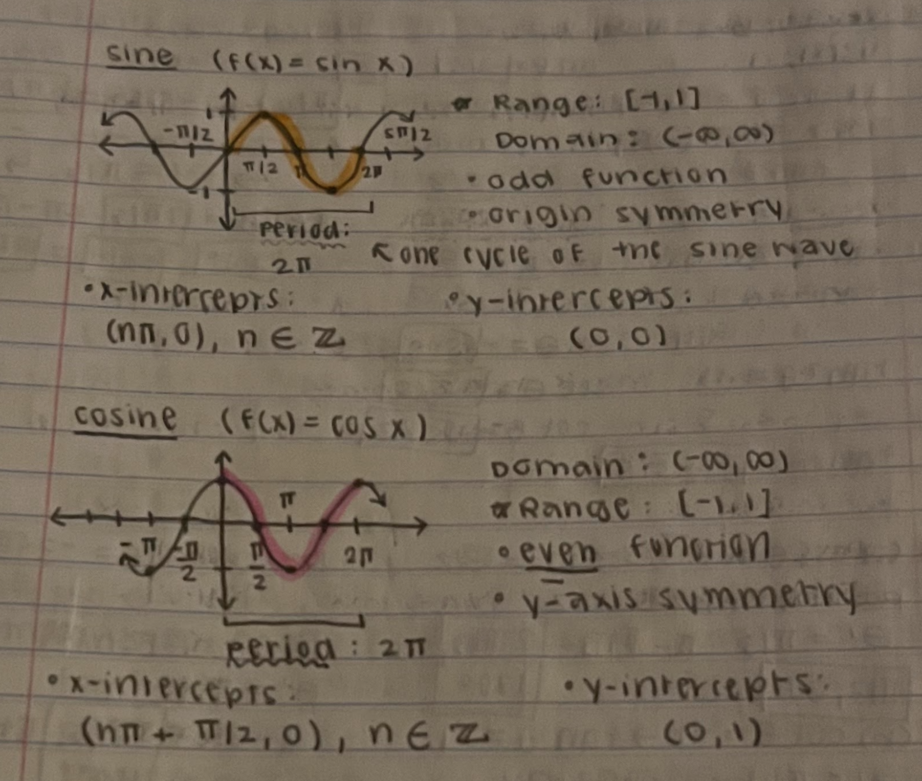
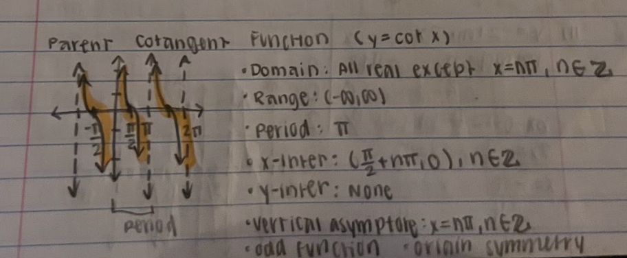
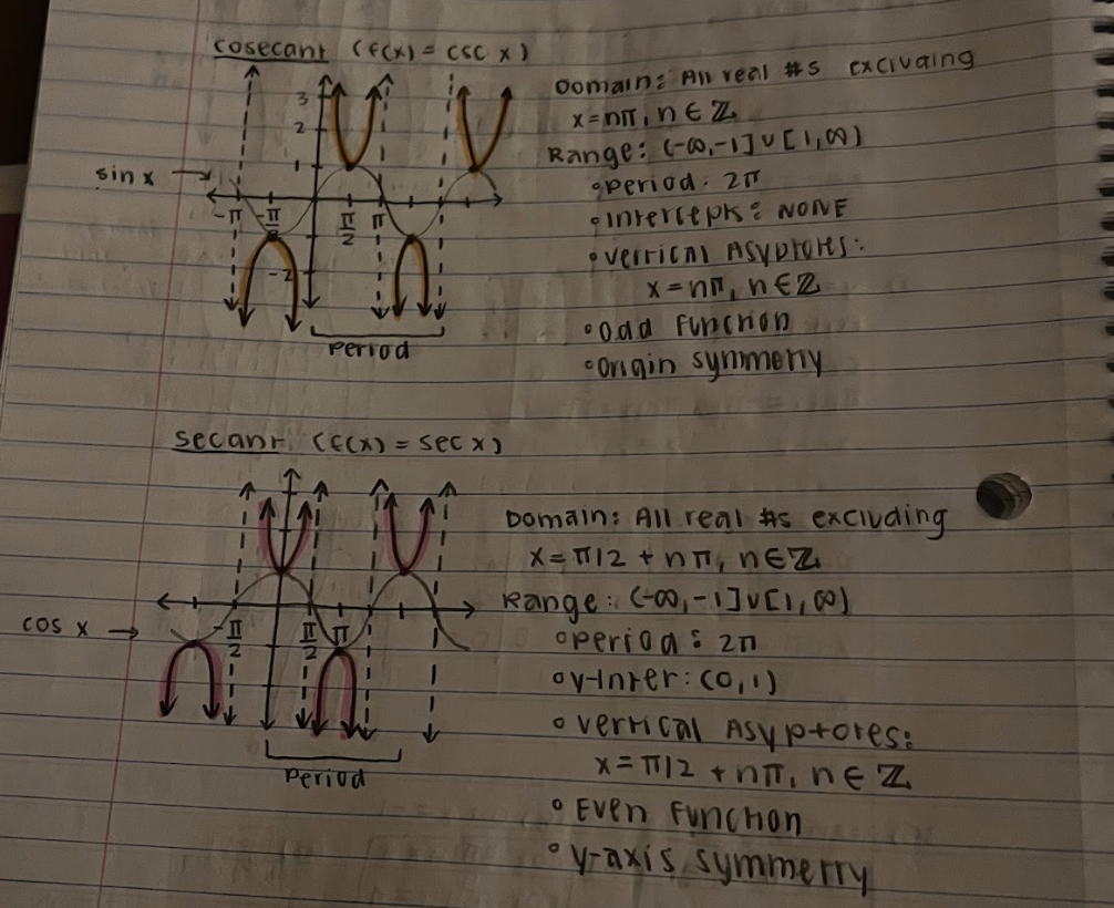
Parent Graphs
Sine Formula: y = a(sin(bx - c)) + d
Cosine Formula: y = a(cos(bx - c)) + d
Amplitude: (a) half of the distance between min/max values
Period (T) = 2π / b
Phase Shift = c / b
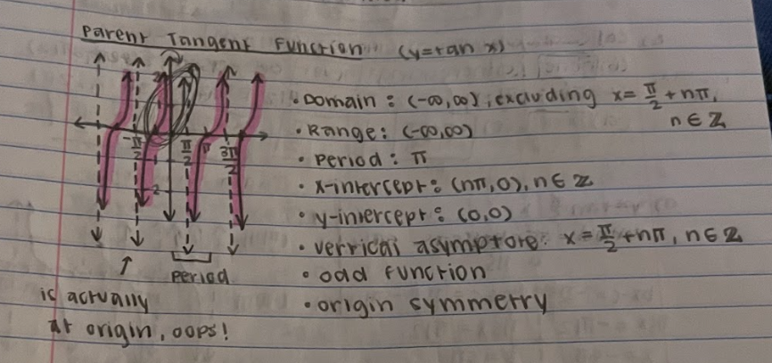 **MISTAKE: The midpoint of one tangent cycle is at the origin
Inverse Trig Function | Domain | Range |
|---|---|---|
y = arcsin x | [-1, 1] | [-π/2, π/2] → Q1 & Q4 |
y = arccos x | [-1, 1] | [0, π] → Q1 & Q2 |
y = arctan x | (-∞, ∞) | (-π/2, π/2) → Q1 & Q4 |
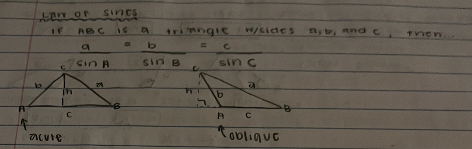
Law of Sines
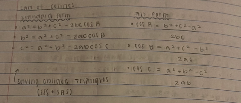
Law of Cosines
Ch. 9 - Parametric & Polar Functions
Eliminating the Parametric
In one parametric equation, solve for t
Substitute the equation for t in the other equation
Simplify
Polar Coordinates

Coordinate Conversion
sin θ = y / x
cos θ = x / r
tan θ = y / x
Polar-to-Rectangular
x = r(cos θ)
y = t(sin θ)
Rectangular-to-Polar
tan θ = y / x
x2 + y2 = r2
Testing for Symmetry in Polar Equations
Over line θ = pi/2: replace (r, θ) by (r, θ-π) or (-r, -θ)
The polar axis: replace (r, θ) by (r, -θ) or (-r, π-θ)
The pole: replace (r, θ) by (r, π+θ) or (-r, θ)