psyc3010
lecture 1
intro to factorial designs
review:
one way designs
- are the means from each level of the factor different from the grand mean (each other)
- independent t test
- one way ANOVA
two way designs
- combine 2 one-way designs using factorial design
- ‘factor’ is categorical independent variable with at least 2 levels
- every factor is crossed
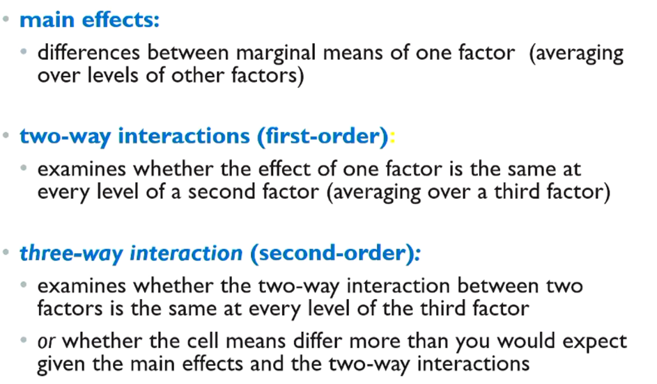
- is there a main effect of factor 1 or 2, or an interaction
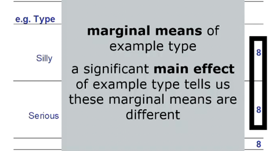
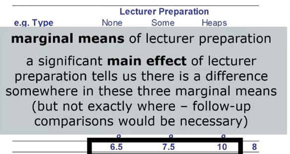
- main effect: are the means of the population corresponding to each level of the factor different?
- intx: does the effect of one factor on the DV change based on the level of another
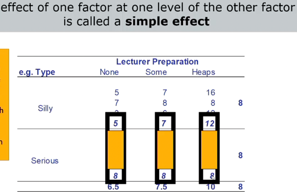
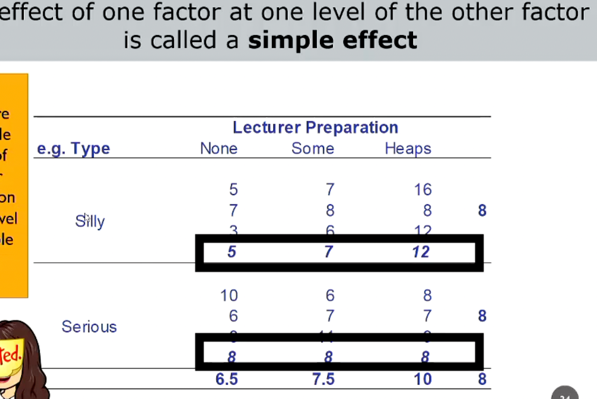
- simple effect: impact of a factor within one level in another factor (cell means)
- two way ANOVA
advantages of factorial designs
- economical (budget) more tests less participants, same power
- allows examination of interactions
- more generalisable
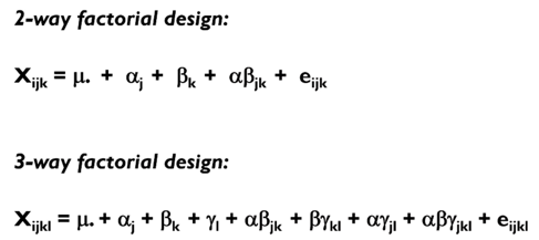
notation in factorial designs
- by no. of factors (two-way between participants)
- by no. of levels in each factor (2x3 between participants)
- 6 cells in 2x3 design
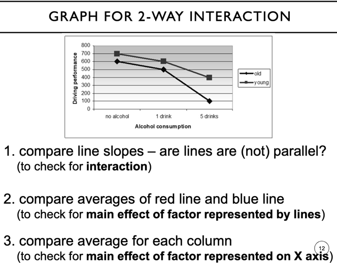
plotting main effects and interactions
- y axis for dependent variable
- x axis for factor with most levels or factor which is most important
- other factor represented by different lines
- all cell means must be represented
- parallel lines = no interaction
- non-parallel = interaction
- main effect = difference in average heights of line and column factor

df
for 3 x 2 x 3 design
df for a = 2, b =1, c = 2
df for ab intx =2
df for ac intx = 4
df for bc = 2
df for abc = 4
error = n-12
lecture 2
factorial between Ps ANOVA 1, omnibus tests
conceptual basis of ANOVA
- analysing, partitioning variance
- if variation due to conditions is greater than variation due to error
- variance: spread of scores around mean
- always some variability
- error variance cannot be explained (random or unmeasured variables)
- treatment variance: systematic differences due to IV
- total variation made up of
- within-groups variance (error/unmeasured influence)
- sum of squared differences between individual scores and group mean
- between-groups variance
- estimate of between groups variability
- almost never 0 difference between groups
- compare ratio of between-groups variance to within-groups variance
- F ratio
- F=MStreat/MSerror
- MStreat: index of variability among treatment means (SSi/DFi)
- MSerror: pooled within-cell variance (SSerror/DFerror)
- estimate of population variance
- large F = reject H0
structural model of one-way ANOVA
- , any DV score, is a combination of
- grand mean + effect of a treatment factor (j) + error for i person in treatment (j)
- expected mean squares
- E(MSerror): long term average of variance in each sample = population variance
- E(MStreat): long term average of between-group variance
two-way factorial ANOVA
- main effects of factor A and B and interactions
- simple effects = same = no interaction
- total variation
- within-groups variance
- between-groups variance
- variance due to factor a
- variance due to factor b
- variance due to interaction
structural model of two-way ANOVA
- , any DV score, is combination of
- grand mean + effect of treatment (j) at factor (A) + effect of treatment (k) at factor (B) + effect of differences in factor A treatments at different levels of factor B treatments + error for (i) person in j and k treatments
assumptions of ANOVA
- population
- treatment populations are normally distributed (normality)
- treatment populations have same variance (homogeneity of variance)
- sample
- independent samples (not RM in this case)
- each sample obtained randomly
- at least 2 observations per sample and equal n
- data
- interval or ratio
lecture 3
between-participants ANOVA 2
significant effects
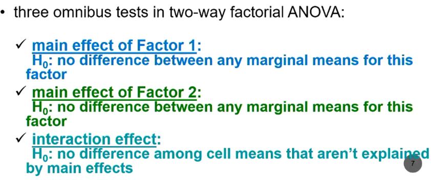
omnibus test (main effects+ interaction)
- always conducted
- outcome of test either supports H0 or H1
- if significant main effect, must interpret and establish direction
- if 2 levels = easy to understand effect direction
- if >2 levels?
- which means differ? where is interaction
- examines interaction, including 2-way and 3 way interactions
- if significant interaction, must interpret direction of simple effects
- differences between levels at one variable same as differences in moderator?
- differences between levels at one variable same as differences in moderator?
main effect comparisons
- which marginal means are different
- t test or linear contrasts
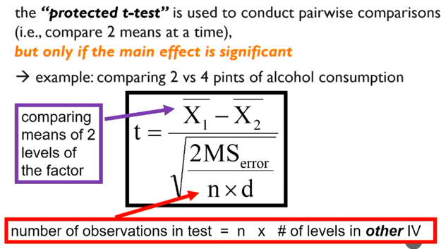
protected t test
- conduct pairwise comparisons
- protects against t1 error
- uses pooled error
linear follow-ups
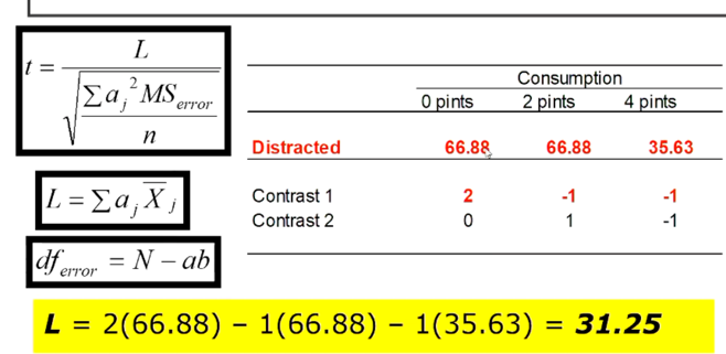
- weighting
- orthogonal contrasts
- weights must add to 0
- rows and columns
pairwise comparisons
Bonferroni correction
- divides p value by no. of comparisons
- adjusts for t1 error by changing crit. value of tests
- higher p value for more tests
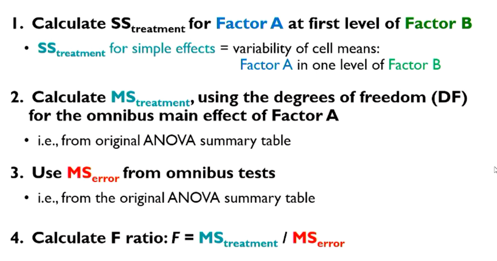
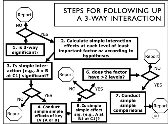
following up interactions (simple effects)
- significant interaction must always be followed up by tests of simple effects
- effect of 1 factor at all levels of another factor
- note that higher order interactions may require changing of interpretation of initial lower/main effects
- esp. if disordinal interaction (no main effects but simple effects in opposite directions)
- testing simple effects:
- sum of simple effects of factor A at each level of factor B = sum of main effect of factor A + interaction (and vice versa)
- simple (effect) comparisons
- follow up significant simple effect with more than 2 levels
- significant simple effect = at least 1 sig. difference between the levels of condition
- use either t tests, F, or linear contrasts
- orthogonal contrasts: variance is partitioned without overlap, use different portions of variance to avoid inflating t1 error
- have as many contrasts as are in the df for the effect (3 levels of condition = 2)
- multiply contrast weight and cell mean
- same as main effect comparisons, but compare cell means rather than marginal means
- not reported for non-sig. simple effects
effect sizes
- problem with p values
- dichotomy: significant or non-significant
- arbitrary acceptance criterion
- larger samples often result in significance
- no info about practical significance of findings
- proportion of variance accounted for
- effect size ‘Cohen’s d’ for t test
- able to compare absolute effects attributable to different variables
- kind of arbitrary cutoffs (small = 2%, med = 16%, large = 24%)
- cutoffs depend on what field of psychology
- effect sizes in anova
- eta squared (η2)
- proportion of variance in sample DV accounted for by effect
- easy to interpret, most common
- biased estimate of true variance in population
- sseffect (e.g. AxB) /sstotal
- omega squared
- proportion of variance in population accounted for by effect
- less biased, more conservative
- however usually same or similar to eta squared depending on sample size (if n = >20)
- larger error variance, smaller sample size = bigger diff. between eta and omega sq
- (sseffect-(dfeffectxMSerror))/sstotal+MSerror
- partial effect sizes
- partial eta squared (pη2)
- proportion of total variance (residual variance) accounted for by investigated effect
- model removes variance attributable to other effects + interaction
- compare variable A to variance attributable to A + error
- inflated, gives larger effect size
- values for each effect are not comparable (and may add up to >1), cannot make meaningful comparisons
- useful only when only have controls and 1 focal IV but often still report n2
- partial omega squared
tut 2
F-value
- more variance should be attributable to treatment for difference to be significant
- ratio of treatment to error variance
- F <1 = non significant
- means error var > treatment var
between-groups variance
- = variance due to factor A + variance due to factor B + variance due to interaction
lecture 4
between-subjects ANOVA 3
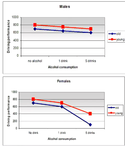
higher-order designs
- design with higher external validity
- e.g. 2x3x2 design (age, alcohol, gender on driving performance)
- 3 possible main effects
- 3 possible 2-way interactions
- averaged across third factor
- averaged across third factor
- possible 3 way interaction
- two-way interaction changes depending on presence of 3rd factor
- plot 2-way interactions at each level of 3rd factor
- if graph for AB at C1 is different from AB at C2, there is an interaction
main effect comparisons
- significant simple effect for factor >2 levels = t-test or linear contrast as in 2 way ANOVA
- simple interaction = f test (omnibus)
- use different error terms
- simple simple effects
- follow up after significant simple effect finding 3-way interaction
- examine each factor of IV at every combination of 2 moderator factor levels
- 1 test at every level (2x3x2 = 6 tests for 1st level of IV)
- uses pooled error term (MS error from omnibus ANOVA table)
- same error term for every omnibus test and follow-up
- contrasts
- simple simple comparisons
- follow up significant simple simple effects with >2 levels
- t test and linear contrasts
- comparing differences
- however
- too many tests = t1 error
lecture 5
power analysis and blocking designs
review of 3-way ANOVA
- omnibus tests
- main effects
- two-way interactions
- three-way interactions
power analysis
- probability of correctly rejecting hypothesis
- = 1-B
- only applies to reality where effect is real
- purposes of power
- making sure you have enough power in study to detect a predicted effect
- or did not find a significant effect although a difference exists in the population; power must be increased to detect it
- increasing power
- change (lower) alpha
- this may make t1 error more likely
- increase IV effect size
- increase sample
- reduce error
- significance testing in ANOVA
- f obtained is compared to f critical
- f = effect of IV (aka difference in group means) / error variance
- how to reduce error variance
- improve power with SALE: increase sample, increase a level, focus on larger effects, decrease variance
- improve operationalisation of variables
- improve measurement of variables
- improve design
- improve methods of analyses
- a priori estimation of effect size
- estimation of effect size and error variance from previous research
- estimate error (MSerror)
- what N is needed to achieve a power of 0.8
- post-hoc estimates
- gather effect size, MSerror, and N from own study
- effect size (Cohen’s d)
- closely related to power
- overlap of distributions between groups
blocking designs
- introduce control variable (concomitant variable) that will account for variance in DV
- thus taking it out of error term
- increasing power by decreasing error variance
- reflects other sources of variation or preexisting differences on DV score
- e.g. studying teaching style effect on problem solving: control variable = IQ
- how to set up
- divide people into groups (blocks) according to control variable (e.g. IQ) known to be associated with DV
- people within blocks each randomly assigned to different levels of IV
- stratified random assignment
- partition variance
- variance from IV
- variance from control
- main effect of blocking = good control variable
- variance from error
- variance from IV * control
- bad, sign of confound
- also detects potential confounds
- benefits
- may equate treatment groups better (assuming equal n for blocking levels)
- more power
- can check interactions of treatment and blocks
- limits
- more expensive
- loss of power if blocking variable is not correlated with DV (fewer df error, higher fcrit)
- artificial grouping due to arbitrary levels of blocking IV may result in loss of information
tut 4
manipulation checks
- purpose
- check whether IV manipulation is actually effective
- did participants experience IV levels in way intended
- or is difference in DV due to another confounding factor
- develop measures to check effectiveness of manipulations
- look at marginal means to determine main effect and direction of manipulation (MMs should be higher for 2nd level)
- hopefully no interaction
lecture 6
bivariate correlation
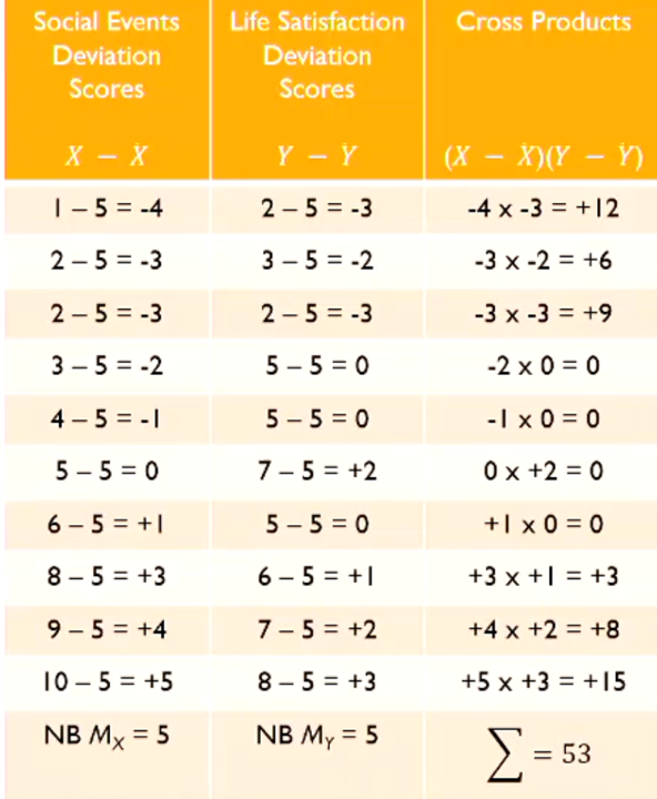
covariance
- multiply together cross products of deviation scores
- is scale dependant
- need scale info to answer questions on association
- numbers from 2 IVs go up/down together = positive cross products, correlation. one goes up another goes down = negative cross products, no correlation
pearson’s r
- relationship between 2 variables in terms of stdevs
- standardised but biased to sample
- rho or radj is population coefficient, compared to r
- average cross product of standardised scores
- r2
- standardised
- tends to be overly liberal (high) with small samples
regression
- estimating scores on variable on the basis of scores of a predictor variable
- “regress DV on IV”
- y = ab+x (or mx+c)
- formula for b is r in correlation
- b is not standardised
- to standardise, change from units to standard deviations
- B = Zscore change in Y predicted by 1 SD increase in X
- b and B can also be tested for significance (t test)
- errors of prediction
- calculate error from line of best fit aka regression line
- regression line fitted in order to fit least squares criterion
- reduce error so that errors of prediction are a minimum
- standard error of estimate
- bigger correlation = smaller SE of e
- how scores are expected to cluster relative to line
- x percent of people expected to be within ~ x SDs of regression line
- underestimated for small samples
- SSy
- = SSregression + SSresidual
- F
- MSregression/MSresidual
ANCOVA
- adding an extra IV that is known to account for changes in DV in a study where there is a large amount of unexplained variance
- covariance is tendency of two scores to vary together
- covariate is continuous control variable known to be associated with DV
- can be applied to any ANOVA design
- same goal as blocking but works differently
- blocking works at level of design
- ANCOVA the error term is adjusted statistically (post hoc)
- control variable can be continuous
- 1st effects of covariate are subtracted from error term, then treatment means are adjusted to account for (remove) differences in covariate
- usually random assignment to IV conditions prevents differences in covariate means (no confound)
- if there isn’t same mean on covariate, it is a confound and removed from data (partial out/control for effects of covariate from focal IV and error term)
if adjusted and observed means are very different, indicates groups differ on covariate in real life and removing these is problematic
- goal is to remove variability on covariate from error term and treatment effect
- this is only done on the assumption there should be no differences in groups due to random assignment
- “would focal IV have effect on DV if all differences due to covariate were removed”
- ANCOVA then tests for differences between adjusted group means
- covariate is like the control variable used for blocking
- however is continuous (i.e. participants not treated at discrete levels)
- should not differ between levels of IV
- reduces error term and increases power
- refines error term (reduces DV) and treatment effect
- previous limitation is that it is post-hoc and increases t1 error
- if covariate unrelated to DV, error term is reduced and power not increased (increases t2 error)
- assumptions of ANCOVA
- same as those of ANOVA
- homogeneity of variance, normal distribution, independent errors
- linear relationship between DV and covariate, overall and within each group
- ANOVA cannot detect non-linear relationships, reduces power
- homogeneity of regression slopes
- no IV x covariate interaction
- relationship between DV and covariate is same in each group
- if not the same, grand slope will be incorrect
- strength
- ability to analyse continuous variables
- splitting into groups causes loss of info and increase in error
- better than blocking if variables are continuous and is applied correctly
lecture 7
correlation and bivariate regression = 1 predictor
multivariate regression
- variation as function of multiple predictors acting together
- predictors are correlated and contribution overlaps
- have to remove overlap to accurately understand effect of variance
- overall relationship between model and predictors (R2) = F test
- can calculate F from R
- importance of individual predictors = b, B, sr
- t test
- confidence intervals
- partial variation (p)
- semipartial variation (spr2) = proportion of variance in DV uniquely explained by IV
linear model (1 predictor) = y = mx+c
linear model (2 predictors) = y = m1x1 +m2x2 +c (plotted on 3D graph)
- aka linear composite
- plane of best fit rather than line of best fit
- least-squares
chronbach’s A
- indicator of internal consistency for 2 items on continuous scale
- how well items hang together
- scales should have A > .7 to reduce error
correlation matrix
- relationship between predictor and DVs ( ties)
- intercorrelations among predictors (collinearities)
- smaller is better, less error
- to maximise R2 should have high validities, low collinearities
- parsimony = IVs explain unique variance
standardised regression coefficient
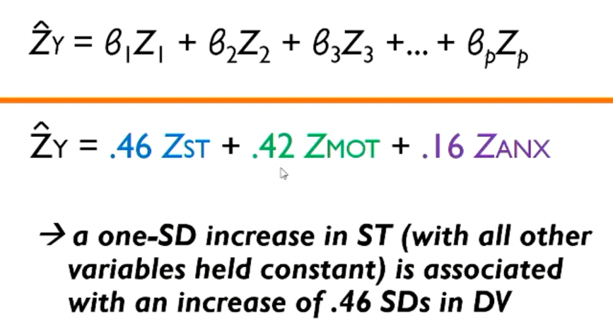
- when IVs not correlated, B = r
- when IVs are correlated
- Bs are affected by correlation among predictors
standard vs hierarchical regression
- standard
- all variables entered simultaneously
- each predictor evaluated in terms of what it uniquely adds to prediction (unique variance)
- model r2 evaluated in 1 step
- hierarchical
- predictors are entered sequentially in prespecified order based on logic/theory
- a priori
- predictors can be entered singly or in blocks
- SPSS outputs r2 and r2 change for each step
- fuller model = variables added, reduced model = without added variables
- r2 change = r2f - r2r
- each predictor evaluated on what it adds to prediction at point of entry
- model r2 assessed in multiple steps
- B is based on current and previous IVs
- useful when looking at old and new variables
lecture 8
multiple regression
assumption of residuals required to perform a multiple regression
- normally distributed
- heteroscedasticity: variance of Y values are consistent across yhat values (homogeneity of variance)
- no linear relationship between yhat and errors of prediction
- independence of errors
multicollinearity and singularity
- occurs when predictors are highly correlated
- leads to type 1 and 2 error
- should delete redundant items
- if not too highly correlated = high parsimony
interactions in multiple regression
- test for regression
- if significant interaction, follow up
- simple slopes of XY lines at different values of Z
- moderator enhances or attenuates relationship between IV/predictor and DV/criterion
- linear model for interaction
- linear regression model has IV and moderator and proposed interaction
- moderated regression asks if XY interaction significantly contributes to prediction of Y
- test this by entering direct effects in block 1, interaction term in block 2
- sig r^2 change in block 2 will determine if interaction is significant
- follow this up by examining simple effects (simple slope analysis)
- relationship of focal IV to DV at diff. level of moderator (usu. low and high)
MMR steps
- centre focal iv and moderator
- reduces multicollinearity
- easier to interpret coefficients when interaction is present
- not scale-dependent
- calculate centred interaction term
- interaction term is part of regression equ.
- must create new variable (IVxmoderater) to create the interaction term to add to equ.
- these must be centred to avoid high collinearity (also makes it easier to interpret coefficients if interaction is present due to same scale)
- subtract mean from original score for each value for both the IV and moderator
- mean for IV and for moderator is 0
- then multiply the centred terms together
- DV is not centred (no collinearity)
- test for significance of interaction
- hierarchical regression analysis
- enter centred IVs in block 1
- interaction term in step 2
- see if this accounts for additional variance not seen in step 1
- IF significant, test simple slopes
- select levels of the moderator to examine
- usu. use +1 and -1 SDs of moderator
- b is gradient for XY when Z=0
- centred variables mean 0 is mean of Z
- recente moderator so me 2 to make moderator go backan is low or high
- to recentre moderator as high, minus one SD from centred (cMod-SD)
- to recenter moderator are as low, add one SD from centred
- then run 2 regression analyses, 1 where moderator is centred low and 1 where it is centred high
- dv x cIV x cModLo
- dv x cIV x cModHi
- interaction should change significantly
- testing and reporting bl (slope)
- then plot simple slopes
lecture 9
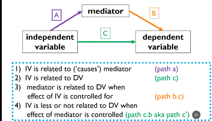
analysis of mediation
- moderation: IV moderates DV (direct relationship)
- mediation: indirect relationships between IV and DV via 3rd variable
- media meaning middle
- cannot be identified via SMR
- \
- IV is related to mediator (path A), (condition 1 of mediation)
- show via SMR
- \
- IV must be associated with DV (condition 2 of mediation)
- HMR
- block 1: predict DV from IV (IV entered)
- block 2: predict DV from IV + mediator (mediator entered)
- path C coefficient should get smaller, partial mediation
- or become non-sig., full mediation
- if yes to both, condition 3 is met
- \
- conduct test of indirect effect
- Sobol test
- bootstrapping
- take sample and assume it was taken from population without bias
- create new samples based on that data
- report results with larger set of data
- uses CI, not p
- criticisms
- can demonstrate path A with just correlation
- significant path C not necessary for indirect effect to be present
- esp. with suppression models
lecture 10
ANOVA
- between participants
- each person in only 1 cell
- assume difference is due to manipulation
- within – cell variability is residual error
- error within a level is the deviation from the group mean
- within participants
- participants serve in multiple treatments
- no within-cell variance
- violates independence assumption of ANOVA
- can calculate and remove variance due to dependence (individual differences)
- decreases error, increases power
- error = inconsistencies in treatment effect for an individual
- <<error used for any effect in RM ANOVA is = to the interaction between that effect and the effect of participants (applies to main and simple effects and their follow up tests)<<
- in a fully within-participants design, every level of factor is tested on every individual
- 1 observation per cell (e.g. person j in condition b)
- no within-cell variance
- error is interaction between treatment factor with participant factor
- compute error term estimating inconsistency as participants change over levels
- every test has own error
- e.g. effect of factor b should be the same across all individuals
- no individual participant variability as every participant only measured once
- note that df is for observations, not participants as participants take place in multiple treatments
- dferror = n-1 * levels(j)-1
- following up main effects
- each comparison must have an error term calculated for it (MSa at b1 *p)
- 2 types of within-participant designs
- mixed model (participant is random factor, treatment is fixed factor)
- random factors have different error terms
- adjustments usually required as assumptions: often violated
- sample is randomly drawn from population
convenience samples
- DV scores are normally distributed in population
- compound symmetry – very restrictive, often violated
homogeneity of variance
homogeneity of covariance
solve via assumption of sphericity
broad and less specific
determines where variance and covariance is roughly equal – is sig. if assumptions are violated
often not sig. when assumptions are violated (not robust)
when does sphericity not matter:
between-participants (as unrelated treatments)
homogeneity of variance still important
when within-participants designs only have 2 levels
only 1 covariance
does matter in within-participants with 3+ levels
if sphericity is violated, F is positively biased (t1 error)
so change Fcrit by adjusting df
‘epsilon adjustment’
e is no. by which Fcrit is multiplied
is 1 when sphericity is not violated
smaller = more conservative
when applied to block, p values change because df changes
- multivariate model (MANOVA)
- creates linear composite of DVs
- RM variable treated as multiple DVs and combined/weighted to maximise difference between levels of other variables
- like how regression combines multiple predictors
- does not have as restrictive assumptions, but more complex to perform
- how it works
- weights DV for each level of the RM IV w/coefficients
- creates predicted DV score that maximises difference across levels of IV
- no adjustment to df required like in RM ANOVA
- uncommon, tends towards t1 error, very specific use case
- report mixed model Fs and GGs, not full MANOVA statistics
- advantages
- very powerful, more sensitive
- simplifies procedure (less people)
- disadvantages of within-participants
- restrictive assumptions
- sequencing effects
- practice
- fatigue
- habituation
- sensitisation
- contrast – previous treatment sets standard to which participant reacts (more broad than sensitisation)
- adaptation – adjustment to previous treatment changes reaction to next (more broad than habituation)
- direct carry-over – learn something in previous trials that is applied to latter ones
- counterbalancing
- req. to reduce sequence effects
- randomise order of treatments if possible
- effect still exists, just reduces bias
- because of this, mixed ANOVA exists to avoid sentencing effects
TUT
regression:
ANOVA: independent variable
regression: direct effect
ANOVA: main effect
regression: simple slope
ANOVA: simple effect
lecture 11
mixed model ANOVA (split-plot ANOVA)
- best way to do WP ANOVA
- has a between participants and within participants factor
- can use non-experimental variables (e.g. brain injury)
- observations are independent, can avoid carry-over and sequencing effects
- assumptions
- homogeneity of variance between groups and levels of factor
- DV is normally distributed in population
- homogeneity of interaction between RM factor and p factor at all levels of WPF
- error for RM factor doesn’t change between groups
- variance-covariance matrix consistency
- variance and covariance are the same at all levels of WPF (often violated)
- epsilon adjustments
- pooled variance-covariance matrix has sphericity
- example
- participants (nested between 3 factor groups: drug, lesion, control) crossed with blocks of learning trials and learning outcome compared
- block (trial) and group are both fixed factors; participant is not fixed
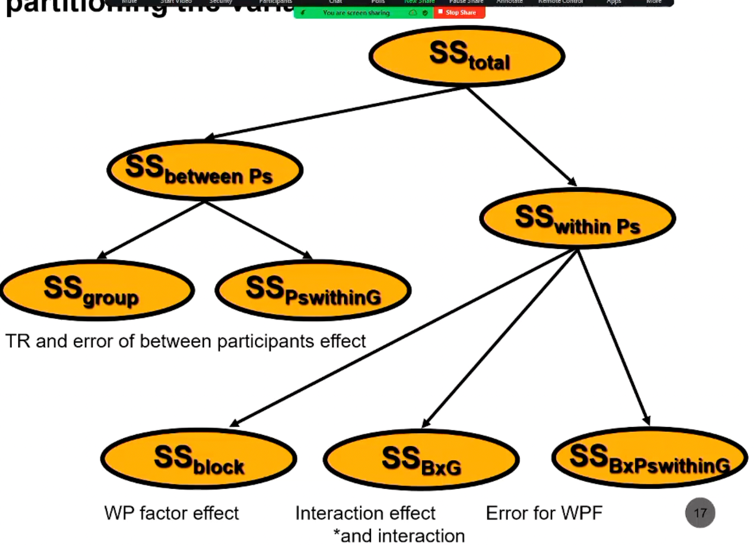
- partitioning of variance
- within participant variability (variance of participant outcome over IV: trials)
- 3 sources
- ss block (RM factor)
- ss bxgroup (interaction)
- ss bxps within g (error for above effects)
- between participants
- ss (whole) group
- ss participants within group (deviation of participants from their group mean)
- 3 omnibus tests
- error terms
- 1 required for p within g factor (between factor)
- 1 for within participants factor and interaction (block x p within g)
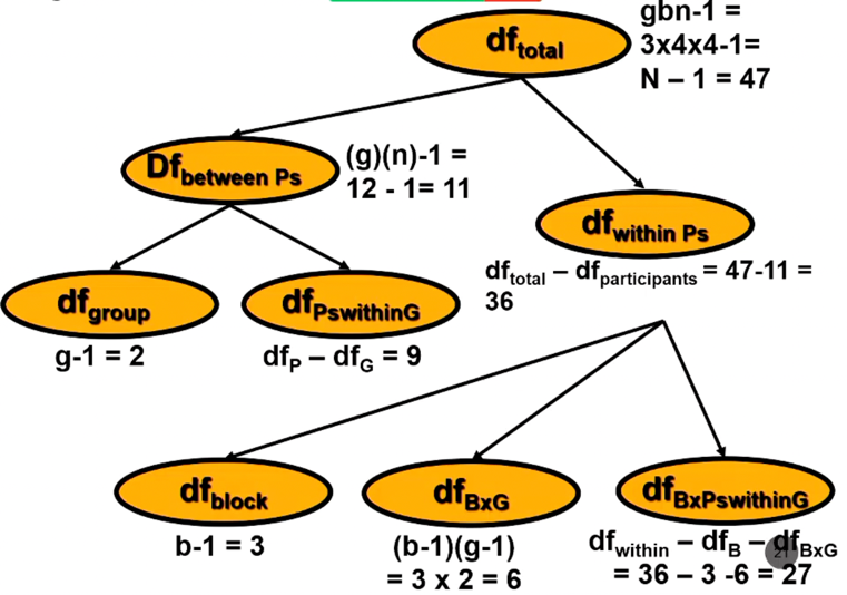
- all df terms add up to dftotal
- following up sig. intx
- between participants
- use error term from between participants main effect (ms ps within g)
- within participants
- separate error term as in MANOVA
- ms bxps within g
- simple effects
- one-way ANOVA of WPF at BPF
- repeat for each block of trials
- each simple effect has own unique error term
- average of simple effect error terms is same as that of MS bxps within g intx
- or pooled error term (MS ps within cell)
- estimate of average error variance within all cells
- should be ok as observations should be independent
- simple comparisons
- ANOVA or linear contrasts depending on what was used for effects
- new error terms used (unless pooled term)
lecture 12
ANOVA
- as opposed to correlational design, can infer causality
- due to random assignment to IV levels
- interaction: effect of A on DV changes over levels of B
general linear model
- system of linear equations used to model data
- versatile and powerful
correlation and t test
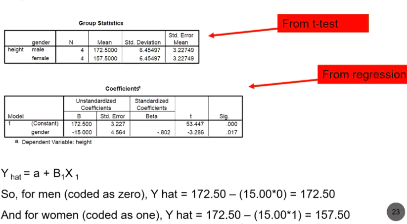
- point-biserial correlation/ independent samples t test
- 1 variable is dichotomous, other is continuous
- can perform ANOVA, linear regression, r or t test, will give same p
- however error will be different
- and regression doesn’t report group means (but can get from unstandardised B)
- regression intx: relationship between X and Y varies over values of Z (moderator)
- 1 variable is dichotomous, other is continuous
hierarchical regression and ANCOVA
- F change in regression is same as ANCOVA
- achieve same broad purpose
- ANCOVA doesn’t give effect sizes (without calculations req.)
increasing power
- ANOVA
- blocking
- improving measurement
- remove individual differences (within ps or RM design)
- include covariate (ANOVA)
- regression
- use of covariate
- improved measurement
TO REVISE FOR EXAM
reading simple effect regression equations (y=mx+v for simple effects)
b vs beta weights
residual / regression variance
split plot ANOVA
error terms ANOVA and regression
compare within and between groups ANOVA
graphing interactions and main effects (and interactions without main effects)
blocking designs
crossing/fixed/random factors/conditions
interaction term means