Comprehensive Economics Notes: Market System, Business Economics, Macroeconomics, and the Global Economy

Unit 1: The Market System

The Basic Economic Problem and Resource Allocation

• Foundational Economic Concepts:

  • Needs: The basic necessities required to sustain human life, such as food, water, clothing, and shelter.

  • Wants: Human desires that exceed basic survival necessities, such as luxury vehicles, high-end electronics, and designer goods.

  • Scarce Resources: Resources that exist in limited quantities and are insufficient to satisfy all human wants.

  • Capital-Intensive Production: A production method relying primarily on machinery, equipment, and automated technology rather than manual labour.

  • Labour-Intensive Production: A production method relying predominantly on human labour rather than capital machinery.

  • Opportunity Cost: The value or benefit of the next best alternative foregone when making a choice.

  • Capital Goods: Goods produced and utilized by firms to manufacture other goods and services, such as plant equipment, factories, and raw materials.

  • Consumer Goods: Goods and services directly consumed by households and individuals to satisfy immediate needs or wants.

  • Production Possibility Curve (PPC): A graphical model illustrating the maximum potential combinations of two products an economy can produce within a given time frame when utilizing all its available resources fully, efficiently, and effectively.

  • Economic Growth: An outward expansion in the productive potential of an economy over a specific time period.

  • Recession / Negative Economic Growth: A contraction or fall in the productive potential or real output of an economy over a period of time.

• The Fundamental Economic Problem:

  • The core economic problem facing humanity is the scarcity of productive resources in contrast to infinite, unlimited human needs and wants.

  • Scarcity forces every society, regardless of political structure, to answer three central resource allocation questions:

  • What to produce?: Deciding which specific goods and services should be allocated resources, prioritizing products essential for meeting survival necessities and basic societal welfare, given that not all desired outputs can be produced.

  • How to produce?: Deciding the optimal combination of inputs and production techniques, specifically choosing between capital-intensive and labour-intensive methods.

  • Who to produce for?: Determining the distribution mechanism of output among individuals and groups within the economy.

Opportunity Cost and Decision-Making

• Principles of Opportunity Cost:

  • Choosing between mutually exclusive options confers an opportunity cost, which is defined as the benefits sacrificed from the highest-ranked alternative that was rejected.

  • Consumer Choice Example:

  • A consumer (Adam) ranks three expenditure options by perceived benefit:

    1. Spending on going to a club.

    2. Spending on travelling the world.

    3. Spending on purchasing a ball.

  • By selecting Option 1, the opportunity cost is specifically Option 2 (travelling the world), as it represents the highest-valued alternative sacrificed.

  • Trade-Offs Across Economic Agents:

  • Governments: Allocating budget funds toward physical infrastructure versus investing in public education.

  • Firms: Choosing whether to direct retained profits into promotional marketing campaigns or salary increments for operational staff.

  • Consumers: Allocating finite disposable income between immediate leisure spending and long-term saving.

The Production Possibility Curve (PPC)

• Interpretation of Points on the PPC Diagram:

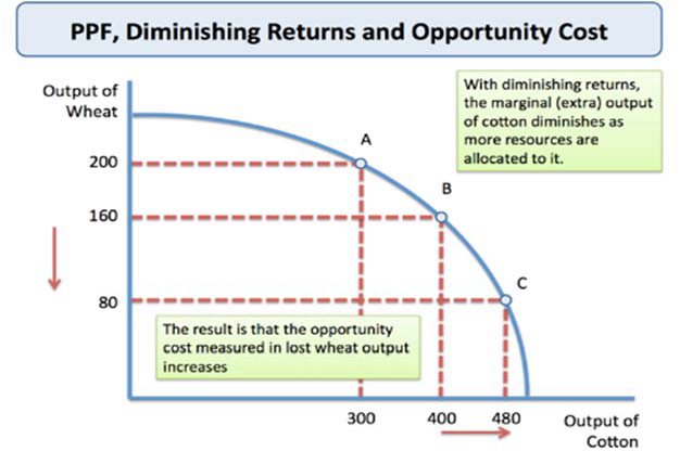
  • Points situated along the frontier curve (such as points $A$, $B$, and $C$) signify productive efficiency, where all available resources are fully employed and utilized at maximum productive potential.

  • Points located strictly inside the frontier curve (such as point $X$) represent inefficient resource allocation, operational underemployment, or idle capacity.

  • Points situated outside the frontier curve (such as point $Y$) are unattainable in the short run given current technology and finite factor endowments.

• Shifts in the Production Possibility Curve:

  • Causes of Outward Shifts (Economic Growth):

  • Introduction and integration of advanced technology, raising overall production efficiency.

  • Adoption of more efficient, streamlined manufacturing and operational methodologies.

  • Increased capital expenditure on worker education and vocational training, improving human capital and labour productivity.

  • Discovery and exploitation of new natural resources, expanding resource availability and enhancing national competitiveness.

• Causes of Inward Shifts (Economic Decline or Recession):

  • Depletion or exhaustion of critical natural resource endowments.

  • Destruction of capital assets, plant machinery, or physical infrastructure caused by natural disasters, geopolitical conflict, or war.

  • Brain drain or a significant decline in the size and health of the active labour force.

  • Prolonged economic mismanagement, chronic underinvestment, or factor obsolescence.

• Diminishing Returns and Increasing Opportunity Cost:

  • Reallocating factor inputs away from one output toward another yields diminishing returns as inputs are not equally suited to producing both goods.

  • Worked Numerical Example:

  • An economy operating on its frontier produces $200\,\text{kg}$ of wheat and $300\,\text{kg}$ of cotton (Point $A$).

  • Moving to Point $B$, the economy produces $160\,\text{kg}$ of wheat and $400\,\text{kg}$ of cotton (reallocating resources yields $+100\,\text{kg}$ of cotton at an opportunity cost of $40\,\text{kg}$ of wheat).

  • Moving further to Point $C$, producing $480\,\text{kg}$ of cotton reduces wheat production to $80\,\text{kg}$ (yielding only $+80\,\text{kg}$ of cotton at an opportunity cost of $80\,\text{kg}$ of wheat).

  • As more resources shift toward cotton, the marginal extra output of cotton diminishes while the opportunity cost measured in foregone wheat accelerates.

Economic Assumptions and Behavioural Realities

• Standard Neoclassical Assumptions:

  • Cost-Benefit Analysis: The evaluation of all anticipated costs and benefits associated with every available choice to select the option that maximizes net benefit.

  • Rational Decision-Making: Consumers and producers act rationally by conducting cost-benefit analyses to maximize utility or welfare.

  • Utility: A metric of the personal satisfaction, well-being, or fulfillment derived from consuming goods and services.

  • Consumer Objective: Consumers aim to purchase the highest quality goods and services at the lowest possible prices to maximize total utility.

  • Producer Objective: Producers aim to manufacture outputs at the lowest possible unit cost and sell them at the highest possible price to maximize total economic profit.

• Reasons Why Consumers Fail to Maximize Utility (Irrational Behaviour):

  • Poor at Computation: Consumers encounter mathematical or analytical difficulty in computing complex net cost-benefit equations, leading to suboptimal product selection.

  • Consumer Inertia: Reluctance to switch from existing service providers or goods despite cheaper market alternatives, driven by fear of unknown risks, switching costs, or perceived lower quality.

  • Habitual Behaviour: Addiction or deep-seated behavioral habits cause individuals to consume items (such as tobacco or alcohol) irrespective of negative welfare effects or escalating prices.

  • Herding: Decisions influenced by peer pressure, family traditions, or social trends, causing consumers to adopt prevailing group habits despite higher financial costs.

  • Feeling Valued / Emotional Attachment: Consumers remain brand loyal (such as emotional allegiance to Nike) due to brand identity, marketing prestige, or perceived status, ignoring cheaper alternatives.

• Reasons Why Producers Fail to Maximize Profit:

  • Principal-Agent Problem: Modern enterprises are frequently managed by hired directors rather than the legal owners (shareholders); managers pursue personal prestige, empire-building, or operational ease rather than pure profit maximization.

  • Charitable Status: Non-profit and philanthropic organizations exist to achieve altruistic social or environmental goals rather than financial profit.

  • Social Enterprises: Commercial businesses operated with the explicit objective of improving societal well-being and reinvesting surpluses into community welfare.

  • Ethical Objectives: Businesses deliberately accept lower profit margins by paying fair trade wages, avoiding sweatshop labor, or utilizing expensive sustainable packaging.

Demand Theory and Market Dynamics

• Definitions in Demand Analysis:

  • Demand: The quantity of a good or service that consumers are willing and able to purchase at various prices over a specific period of time, ceteris paribus.

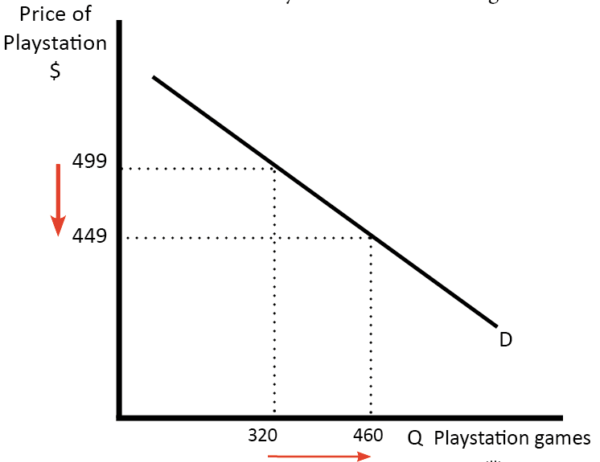
  • Law of Demand: An inverse relationship exists between the price of a product and the quantity demanded: as price ($P$) increases, quantity demanded ($Q_d$) falls; conversely, as price ($P$) decreases, quantity demanded ($Q_d$) rises.

  • Substitutes: Competing alternative goods that satisfy the same consumer desire (e.g., tea and coffee).

  • Complements: Jointly consumed products where the use of one necessitates the use of the other (e.g., tea and sugar; gaming consoles and video games).

  • Consumer Trends: Shifting consumer behaviors, preferences, and purchasing habits over time.

• Movements Along vs. Shifts in the Demand Curve:

  • Movement Along the Curve: Occurs solely due to a change in the price of the good itself, resulting in an expansion (price drop) or contraction (price rise) of quantity demanded.

  • Example: If the price of a gaming console decreases from $\$499$ to $\$449$, the quantity demanded expands from $320$ to $460$ units along the existing curve.

• Shift of the Entire Curve: Occurs when non-price determinants change, shifting the curve rightward (increase in demand) or leftward (decrease in demand) at all price levels.

  • Example: At a price of $60$ pence per can, non-price factors increase demand from $500$ to $600$ units per week, shifting the demand curve from $D$ to $D_1$.

• Non-Price Determinants of Demand:

  • Advertising and Marketing: Increased advertising expenditure elevates brand recognition and perceived value, shifting demand rightward.

  • Consumer Income: Rising real incomes expand purchasing power, increasing demand for normal goods while reducing demand for inferior goods.

  • Changes in Tastes, Fashions, and Preferences: Modern societal shifts, such as social media connectivity, expand the demand for personal digital devices.

  • Price of Substitute Goods: A fall in the price of a substitute good makes it relatively more attractive, shifting demand for the alternative good leftward.

  • Price of Complementary Goods: An increase in the price of a complementary good increases the joint cost of consumption, shifting demand for the associated product leftward.

  • Demographic Changes:

  • Age Distribution: An ageing population shifts demand toward elder-care facilities and pharmaceuticals.

  • Ethnicity: Increasing ethnic diversity expands demand for specialized cultural foods and services.

  • Gender Distribution: Regional variations in gender balance alter demand patterns for specialized consumer goods.

  • Geographic Distribution: Urbanization shifts aggregate demand toward urban transport, compact housing, and municipal services.

Supply Theory and Market Dynamics

• Definitions in Supply Analysis:

  • Supply: The total quantity of a good or service that producers are willing and able to offer for sale at various price levels over a given time period.

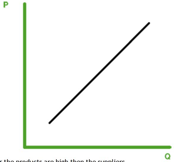
  • Law of Supply: A direct relationship exists between the price of a product and the quantity supplied: higher prices provide greater profit incentives, inducing producers to expand output, whereas lower prices diminish potential returns, causing producers to restrict supply.

  • Costs of Production: The total expenditures incurred by an enterprise to acquire factor inputs and manufacture output ready for distribution.

  • Indirect Taxes: Compulsory levies imposed on the production or expenditure of goods and services (e.g., VAT, excise duties).

  • Subsidies: Government financial grants allocated to businesses to lower unit production costs and encourage increased output.

• Movements Along vs. Shifts in the Supply Curve:

  • Movement Along the Curve: Triggered exclusively by changes in the market price of the good itself, representing an expansion or contraction in quantity supplied.

  • Example: When the price per dozen rises from $\$6$ to $\$12$, quantity supplied expands from $6$ to $12$ dozen units.

• Shift of the Entire Curve: Triggered by changes in non-price conditions of supply, shifting the curve rightward (increase in supply) or leftward (decrease in supply).

  • Example: A rightward supply shift from $S$ to $S_1$ causes market equilibrium price to drop from $P$ to $P_1$ while equilibrium quantity expands from $Q$ to $Q_1$.

• Non-Price Determinants of Supply:

  • Costs of Production: Elevated raw material prices, component expenses, or wage demands diminish profit margins and contract operational liquidity, shifting supply leftward.

  • Indirect Taxation: Imposing or increasing indirect taxes raises production expenses, shifting supply leftward. Governments implement these levies to raise public funds and discourage the production of harmful goods (such as tobacco).

  • Government Subsidies: Providing subsidies via direct cash grants, rent-free facilities, or tax allowances lowers marginal costs, shifting supply rightward.

  • Natural and Environmental Factors: Agricultural yields depend on seasonal conditions and weather events; favorable weather expands crop harvest, whereas droughts shift supply leftward.

  • Technological Innovation: Upgraded manufacturing technology elevates factor productivity, reduces wastage, exploits economies of scale, and shifts supply rightward.

Market Equilibrium and Price Mechanism

• Definitions in Market Equilibrium:

  • Equilibrium Price (Market Clearing Price): The precise price level where market demand equals market supply ($Q_d = Q_s$), leaving neither shortages nor unsold stock.

  • Total Revenue ($TR$): The gross earnings generated from output sales, calculated as:

$TR = P \times Q$

• Market Determination Table (Cap Market Example):

| Price () | Supply (Units) | Demand (Units) | Market Condition | State of Equilibrium |\n| :--- | :--- | :--- | :--- | :--- |\n| `\$20$` | `$100$` | `$200\,\text{Caps}$` | Excess Demand ($100) | Disequilibrium (Shortage) |\n| `\$30$` | `$150$` | `$150\,\text{Caps}$` | Market Cleared ($Q_s = Q_d) | Stable Equilibrium |\n| `\$45$` | `$200$` | `$100\,\text{Caps}$` | Excess Supply ($100) | Disequilibrium (Surplus) |\n| `\$50$` | `$250$` | `$50\,\text{Caps}$` | Excess Supply ($200) | Disequilibrium (Surplus) |\n\n* **Graphical Representation of Equilibrium:**\n * A market clears at the intersection of downward-sloping demand and upward-sloping supply.\n * *Example:* At a price of `£0.35$`, equilibrium quantity transacted equals `$250` units.\n\n\n\n* **Shifts in Simultaneous Curves:**\n * When both the demand curve and the supply curve shift to the right, equilibrium moves from an initial point to a new clearing point. The resulting equilibrium price drops from P_1$to$P_2 as supply expansion outpaces demand growth.\n\n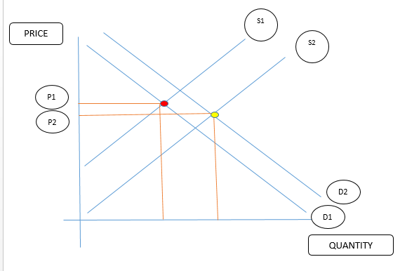\n\n* **Market Disequilibrium:**\n * **Excess Demand (Shortage):** Occurs when the prevailing market price is below equilibrium, causing quantity demanded to exceed quantity supplied (Q_d > Q_s).\n * *Elimination Strategy:* Suppliers raise prices, rationing demand and incentivizing an expansion in quantity supplied.\n * **Excess Supply (Surplus):** Occurs when the market price exceeds equilibrium, causing quantity supplied to outstrip quantity demanded (Q_s > Q_d).\n * *Elimination Strategy:* Suppliers reduce prices and utilize marketing promotions to clear excess inventories.\n * *Diagram Analysis:* At a price of `\text{Rs}\,12$`, quantity supplied is `$6$` while quantity demanded is `$2$` (yielding an excess supply of `$4$` units). At a price of `$\text{Rs}\,2$`, quantity demanded is `$7$` while quantity supplied is `$1$` (yielding an excess demand of `$6$` units). The market clears at$P_e = \text{Rs}\,8$and$Q_e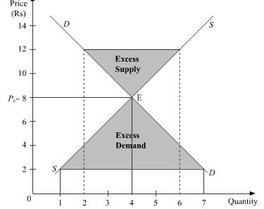 = 4.\n\n\n\n### Price Elasticity of Demand (PED)\n\n* **Definitions and Mathematical Formula:**\n * **Price Elasticity of Demand (PED):** A quantitative measure of the responsiveness of the quantity demanded of a good to a change in its price.\n * **Formula:**\n\nPED = \frac{\%\,\text{Change in Quantity Demanded}}{\%\,\text{Change in Price}}\n\n\%\,\text{Change in Price} = \left( \frac{P_{\text{new}} - P_{\text{old}}}{P_{\text{old}}} \right) \times 100\n\n\%\,\text{Change in Quantity Demanded} = \left( \frac{Q_{\text{new}} - Q_{\text{old}}}{Q_{\text{old}}} \right) \times 100\n\n * *Sign Note:* Due to the law of demand, calculated PED coefficients are naturally negative. When determining elasticity classifications, the negative sign is traditionally ignored (taking the absolute value).\n\n* **Worked Mathematical Example:**\n * The market price of a ball rises from `\$400$` to `$\$450$`, causing quantity demanded to contract from `$20$` to `$15` balls:\n * Step 1: Percentage Change in Price:\n\n\%\,\Delta P = \left( \frac{450 - 400}{400} \right) \times 100 = +12.5\% \n\n* Step 2: Percentage Change in Quantity Demanded:\n\n\%\,\Delta Q_d = \left( \frac{15 - 20}{20} \right) \times 100 = -25.0\% \n\n* Step 3: Calculation of PED:\n\nPED = \frac{-25}{+12.5} = -0.5\n\n * Because the absolute value is less than 1, demand is classified as price inelastic.\n\n* **Numerical Classifications of PED:**\n * **Inelastic Demand (|PED| < 1):** The percentage change in quantity demanded is proportionately smaller than the percentage change in price.\n\n\n\n* **Elastic Demand (|PED| > 1):** The percentage change in quantity demanded is proportionately greater than the percentage change in price.\n\n\n\n* **Unitary Elastic Demand (|PED| = 1):** The percentage change in quantity demanded is identical to the percentage change in price.\n* **Perfectly Price Inelastic Demand (PED = 0):** A change in price causes zero change in quantity demanded (represented by a vertical curve).\n\n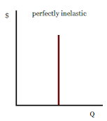\n\n* **Perfectly Price Elastic Demand (PED = \infty):** Any increase in price drops demand to zero (represented by a horizontal curve).\n\n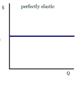\n\n* **Elasticity Along a Downward-Sloping Linear Demand Curve:**\n * Moving down a straight-line demand curve, elasticity declines continuously:\n * Upper Intercept (Red Point): PED = \infty (Perfect elasticity).\n * Upper Segment (Blue Point): |PED| > 1 (Elastic).\n * Midpoint (Yellow Point): |PED| = 1 (Unitary elasticity).\n * Lower Segment (Purple Point): |PED| < 1 (Inelastic).\n * Lower Intercept (Black Point): PED = 0 (Perfect inelasticity).\n\n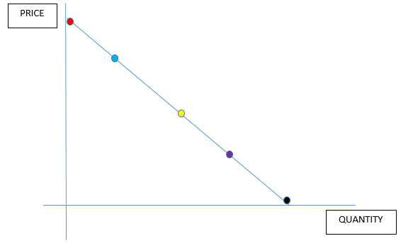\n\n* **Determinants of Price Elasticity of Demand:**\n * **Availability of Substitutes:** Goods with close, easily accessible alternatives exhibit elastic demand; absence of substitutes causes inelastic demand.\n * **Degree of Necessity:** Essential items (e.g., life-saving medicines, staple foods) have price inelastic demand; luxury non-essentials have price elastic demand.\n * **Proportion of Income Expended:** Products absorbing a substantial percentage of consumer income (e.g., cars) exhibit elastic demand; low-cost items (e.g., salt, matches) have inelastic demand.\n * **Time Horizon:** In the short run, consumer demand is inelastic due to informational delays and habit persistence; in the long run, consumers identify alternatives, making demand elastic.\n\n* **Total Revenue and PED Relationships:**\n\n| Price Elasticity Classification | Absolute Numerical Value | Direction of Price Change | Impact on Total Revenue (TR) |\n| :--- | :--- | :--- | :--- |\n| Inelastic | Less than 1 | Price Increase | Total Revenue Increases |\n| Inelastic | Less than 1 | Price Decrease | Total Revenue Decreases |\n| Elastic | More than 1 | Price Increase | Total Revenue Decreases |\n| Elastic | More than 1 | Price Decrease | Total Revenue Increases |\n\n* **Worked Revenue Examples:**\n * *Elastic Product (Sports Balls):* Price drops from `\$8$` to `$\$5$`; sales expand from `$100$` to `$200` units.\n * Initial Revenue: `TR_1 = \8 \times 100 = \800`\n * Final Revenue: `TR_2 = \5 \times 200 = \1000`\n * Result: For an elastic product, lowering price increases total revenue.\n * *Inelastic Product (Bottled Water):* Price drops from `\$7$` to `$\$5$`; sales expand marginally from `$200$` to `$210` units.\n * Initial Revenue: `TR_1 = \7 \times 200 = \1400`\n * Final Revenue: `TR_2 = \5 \times 200 = \1000$` (or `$\5 \times 210 = \1050`)\n * Result: For an inelastic product, lowering price causes total revenue to fall.\n\n### Price Elasticity of Supply (PES)\n\n* **Definitions and Mathematical Formula:**\n * **Price Elasticity of Supply (PES):** A metric evaluating the responsiveness of the quantity supplied of a product to a change in its selling price.\n * **Formula:**\n\nPES = \frac{\%\,\text{Change in Quantity Supplied}}{\%\,\text{Change in Price}}\n\n* **Worked Mathematical Example:**\n * The market price of agricultural vanilla pods rises from `\$2$` to `$\$3$`; market supply expands from `$250$` to `$275` pods:\n * Step 1: Percentage Change in Quantity Supplied:\n\n\%\,\Delta Q_s = \left( \frac{275 - 250}{250} \right) \times 100 = 10\% \n\n* Step 2: Percentage Change in Price:\n\n\%\,\Delta P = \left( \frac{3 - 2}{2} \right) \times 100 = 50\% \n\n* Step 3: Calculation of PES:\n\nPES = \frac{10}{50} = 0.2\n\n * Because the numerical coefficient is less than 1, supply is price inelastic.\n\n* **Numerical Classifications of PES:**\n * **Inelastic Supply (PES < 1):** Quantity supplied changes by a smaller percentage than price.\n * **Elastic Supply (PES > 1):** Quantity supplied changes by a larger percentage than price.\n\n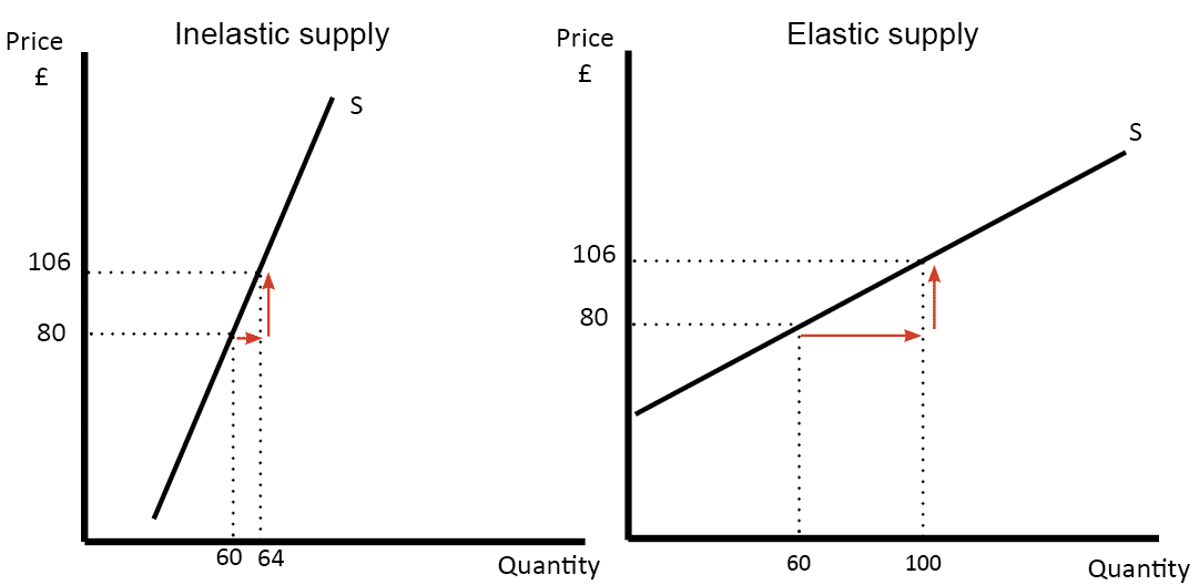\n\n* **Unitary Elastic Supply (PES = 1):** Percentage change in quantity supplied equals the percentage change in price (a linear ray from the origin).\n* **Perfectly Inelastic Supply (PES = 0):** Supply is fixed and incapable of responding to price movements (vertical curve).\n* **Perfectly Elastic Supply (PES = \infty):** Producers supply an infinite amount at a given price, but zero at any price below (horizontal curve).\n\n\n\n* **Determinants of Price Elasticity of Supply:**\n * **Availability of Factor Inputs:** Plentiful, low-cost raw materials allow rapid output expansion, rendering supply elastic.\n * **Stock Storage Capacity and Perishability:** Perishable agricultural products cannot be stored long-term without high refrigeration expenses, resulting in inelastic supply. Durable manufactured goods that are easily warehoused yield elastic supply.\n * **Spare Production Capacity:** Producers with idle machinery and underutilized factory capacity adjust output quickly to price spikes, making supply elastic.\n * **Production Time Lags:** Goods requiring extended production cycles (such as seasonal crops) have highly inelastic supply in the short run. Manufactured Fast-Moving Consumer Goods (FMCG) can increase factory output via overtime labor, making supply elastic.\n\n### Income Elasticity of Demand (YED)\n\n* **Definitions and Mathematical Formula:**\n * **Income Elasticity of Demand (YED):** Measures the responsiveness of demand for a good to changes in consumer real income.\n * **Formula:**\n\nYED = \frac{\%\,\text{Change in Quantity Demanded}}{\%\,\text{Change in Income}}\n\n* **Worked Mathematical Example:**\n * Average annual income per capita rises from `\$5000$` to `$\$7500$`; household milk consumption expands from `$4$` to `$5` bottles:\n * Step 1: Percentage Change in Quantity Demanded:\n\n\%\,\Delta Q_d = \left( \frac{5 - 4}{4} \right) \times 100 = 25\% \n\n* Step 2: Percentage Change in Income:\n\n\%\,\Delta Y = \left( \frac{7500 - 5000}{5000} \right) \times 100 = 50\% \n\n* Step 3: Calculation of YED:\n\nYED = \frac{25}{50} = 0.5\n\n* **Classification of Goods by YED Value:**\n * **Normal Goods (0 < YED \le 1):** Demand increases as income increases, but at a rate equal to or less than proportional income growth (e.g., milk, basic clothing).\n * **Luxury Goods (YED > 1):** Demand expands disproportionately faster than the rise in income (e.g., international travel tickets, sports cars, jewelry).\n * **Inferior Goods (YED < 0):** Demand decreases as income rises, as consumers switch to premium alternatives (e.g., supermarket own-label budget brands).\n\n* **Strategic Significance of PED and YED:**\n * **For Commercial Businesses:**\n * *PED:* Assists managers in revenue forecasting when considering price adjustments. Lowering prices for elastic goods increases gross receipts; raising prices for inelastic goods maximizes earnings.\n * *YED:* Facilitates forward product portfolio planning across economic cycles. During economic booms, firms expand the production of luxury items; during recessions, production shifts toward discount inferior lines.\n * **For Government Authorities:**\n * *Tax Policy:* Fiscal planners impose indirect taxes on price-inelastic commodities (e.g., tobacco, alcohol, fuel) because demand drops marginally, securing stable public tax revenues.\n * *Subsidies and Welfare:* Governments target subsidies toward essential goods with low elasticities to ensure affordability for lower-income households.\n\n### Mixed Economies, Market Failure, and Public Goods\n\n* **Economic Classifications:**\n * **Free Market / Enterprise Economy:** Resource allocation is determined entirely by private firms and consumer price signals through market supply and demand, with minimal public intervention.\n * **Command Economy:** The state owns all factors of production; central planners determine what, how, and for whom to produce.\n * **Mixed Economy:** An economic system combining private market enterprise and public sector intervention to allocate resources (e.g., Saudi Arabia, UK).\n\n* **Ownership and Objectives in a Mixed Economy:**\n * **Private Sector:**\n * *Structures:* Sole traders (single owner), partnerships (2 to 20 owners), and limited liability joint-stock companies owned by shareholders.\n * *Aims:* Commercial survival, profit maximization, profit satisficing, brand growth, and corporate social responsibility.\n * **Public Sector:**\n * *Structures:* Central government ministries, municipal local authorities, public service corporations, and nationalized institutions (e.g., central banks).\n * *Aims:* Public welfare maximization, universal service accessibility, operating cost minimization, internalizing social costs and benefits, and revenue generation from strategic state assets.\n\n* **Market Failure:**\n * Defined as a situation where unregulated private market forces fail to allocate resources efficiently, causing net social welfare losses.\n * **Key Causes of Market Failure:**\n * **External Costs:** Negative externalities (e.g., industrial pollution, traffic congestion) ignored by commercial price mechanisms.\n * **Monopoly Abuse:** Absence of market competition leading to restricted output, high pricing, and consumer exploitation.\n * **Missing Markets (Public Goods):** Total market absence for essential services like national defence and street lighting, because private firms cannot charge non-payers.\n * **Information Failure / Asymmetric Information:** Imbalance of product data between sellers and buyers, leading to poor choices and price gouging.\n * **Factor Immobility:** Inability of factors of production (such as specialized labour or machinery) to move between alternative economic employments.\n\n* **Characteristics of Public Goods:**\n * **Non-Excludability:** Once provided, it is impossible to prevent non-paying individuals from consuming the good.\n * **Non-Rivalry:** Consumption of the good by one individual does not diminish the quantity or quality available for others.\n * **The Free-Rider Problem:** Because non-payers cannot be excluded from consuming non-excludable goods, private individuals refuse to purchase them voluntarily. Private firms cannot profitably price or provide these goods, leaving their provision to the public sector.\n\n### Privatization\n\n* **Definition and Forms:**\n * **Privatization:** The transfer or sale of state-owned enterprises, assets, or operational duties to private commercial enterprises.\n * **Methods of Execution:**\n * *Sale of Nationalized Industries:* Fully selling state enterprise equity directly to private buyers or public stock markets.\n * *Contracting Out:* Inviting competitive tenders from private firms to deliver public services (e.g., municipal refuse collection, hospital cleaning).\n * *Sale of State Land and Property:* Selling public real estate and municipal buildings directly to private citizens or developers.\n\n* **Motivations for Privatization:**\n * Generating short-term fiscal revenue to finance state projects without raising general taxation.\n * Enhancing operational efficiency by introducing commercial profit incentives and competitive market discipline.\n * Reducing political interference and bureaucratic delays in operational and capital allocation decisions.\n\n* **Socioeconomic Effects of Privatization:**\n\n| Economic Agent | Positive Consequences | Negative Consequences |\n| :--- | :--- | :--- | \n| **Consumers** | Improved operational efficiency, potential innovation, enhanced service quality. | Risk of private monopoly pricing, reduction of loss-making essential services. |\n| **Workers** | Performance-linked pay, adoption of flexible modern work practices. | Large-scale redundancies, reduced job security, downward pressure on wages. |\n| **Businesses** | Freedom to pursue profit maximization, commercial expansion, and diversification. | Exposure to hostile takeovers, heightened competitive pressure, cost-cutting risks. |\n| **Government** | Immediate cash receipts from asset sales, removal of chronic state subsidies. | High transactional flotation costs, loss of recurring future dividend revenue. |\n\n### Externalities and Corrective Intervention\n\n* **Taxonomy of Externalities:**\n * **Negative Externality:** Detrimental spillover effects imposed on uncompensated third parties resulting from private production or consumption decisions.\n * *Private Cost:* Direct expenses borne by producers (e.g., raw materials, wages) or consumers (e.g., market price).\n * *External Cost:* Negative side-effects inflicted on third parties (e.g., atmospheric pollution, health degradation, industrial noise).\n * *Social Cost:* The aggregate burden borne by society, defined as:\n\n\text{Social Cost} = \text{Private Cost} + \text{External Cost}\n\n* **Positive Externality:** Beneficial spillover effects enjoyed by third parties without financial compensation resulting from private production or consumption.\n * *Private Benefit:* Direct satisfaction or financial profit gained by consumers or producers.\n * *External Benefit:* Unpriced positive advantages enjoyed by external parties (e.g., herd immunity, reduced crime from education).\n * *Social Benefit:* The aggregate benefit realized by society, defined as:\n\n\text{Social Benefit} = \text{Private Benefit} + \text{External Benefit}\n\n* **Sectoral Contexts of Externalities:**\n * **Transport:** Combustion engines generate particulate matter and carbon emissions, accelerating climate change and causing respiratory illnesses, which raises public healthcare expenditure.\n * **Healthcare:** Vaccinating individuals against transmissible pathogens (e.g., COVID-19) prevents disease spread, generating external benefits by reducing workplace absenteeism.\n * **Education:** Higher education provides graduates with technical skills, driving product innovation, reducing societal unrest, and increasing public income tax yields.\n * **Environment:** Over-extracting renewable and non-renewable resources degrades ecosystems, threatening the living standards of future generations.\n\n* **Policy Remedies for Environmental Externalities:**\n * **Pigouvian Indirect Taxation:** Taxes placed on polluting firms increase private production costs, reducing output toward socially optimal levels and raising tax revenues for environmental remediation.\n * **Direct Production Subsidies:** Financial grants to clean energy or merit good providers lower unit costs, reducing consumer prices and expanding consumption.\n * **Fines and Statutory Penalties:** Strict legal sanctions deter environmentally hazardous actions by imposing clear financial penalties on polluters.\n * **Command-and-Control Regulations:** Legal bans, production limits, and consumer protection laws (e.g., emissions standards) directly prevent market abuses.\n * **Tradable Pollution Permits:** Governments issue capped allowances permitting fixed quantities of discharge. Clean firms sell unused quotas at market rates, whereas heavy polluters face high permit purchase costs, creating economic incentives to adopt cleaner production techniques.\n\n---\n\n# Unit 2: Business Economics\n\n### Factors of Production and Economic Sectors\n\n* **The Four Factors of Production:**\n * **Land:** All natural resource endowments supplied by nature, classified into:\n * *Non-Renewable Resources:* Finite resources depleted by extraction (e.g., crude petroleum, mineral coal, iron ores).\n * *Renewable Resources:* Self-replenishing natural assets capable of sustained utilization if managed correctly (e.g., solar energy, timber, wind).\n * **Labour:** The aggregate mental and manual exertion provided by the human workforce, whose collective capabilities constitute human capital.\n * **Capital:** Manufactured aids used to facilitate further economic production, divided into:\n * *Working Capital:* Inventories of unfinished intermediate components, raw materials, and work-in-progress destined for conversion into final products.\n * *Fixed Capital:* Long-lasting productive assets not consumed within the output itself (e.g., factories, industrial robotics, computer networks).\n * **Enterprise / Entrepreneurship:** The specialized human faculty responsible for identifying commercial ventures, committing financial capital, bearing investment risks, and coordinating the other three factors of production.\n\n* **Comparative Production Methods:**\n\n| Production Method | Key Advantages | Key Disadvantages |\n| :--- | :--- | :--- | \n| **Labour-Intensive** | Cost-effective for customized low-volume production; high operational flexibility; human creativity and adaptability. | Human management challenges; vulnerability to absenteeism; requirement for scheduled breaks and paid holidays. |\n| **Capital-Intensive** | Capability for continuous 24/7 operation; uniform precision and quality; reduced managerial complexity. | High initial capital setup costs; operational inflexibility to design changes; workforce demoralization from redundancies. |\n\n* **Structural Classification of Economic Sectors:**\n * **Primary Sector:** Industries focused on extracting or harvesting raw natural assets directly from the earth (e.g., commercial agriculture, mining, forestry, offshore fishing).\n * **Secondary Sector:** Industrial manufacturing enterprises transforming raw commodities into refined semi-finished and finished physical goods (e.g., automobile assembly, chemical processing, textile weaving).\n * **Tertiary Sector:** Commercial entities providing services to households and other enterprises (e.g., banking, corporate legal counsel, accountancy, tourism).\n * **De-Industrialization:** The long-term contraction of secondary manufacturing employment and output relative to the expanding tertiary service sector within advanced industrialized nations.\n * *Causes:* Wealthier consumers dedicating higher marginal income to leisure and entertainment; outsourcing of manufacturing to low-wage economies (e.g., China, Brazil, India); labor displacement through manufacturing automation.\n\n* **Cross-National Sectoral Employment Comparisons:**\n * **Advanced Developed Nation (USA):** Primary Sector: `2\%$`; Secondary Sector: `$23\%$`; Tertiary Sector: `$75\%`.\n * **Emerging Developing Nation (Brazil):** Primary Sector: `23\%$`; Secondary Sector: `$24\%$`; Tertiary Sector: `$53\%`.\n * **Underdeveloped Nation (Nepal):** Primary Sector: `81\%$`; Secondary Sector: `$3\%$`; Tertiary Sector: `$16\%`.\n\n\n\n### Productivity and Division of Labour\n\n* **Productivity Fundamentals:**\n * **Productivity:** The rate of productive output generated per unit of factor input deployed within a specific time period:\n\n\text{Labour Productivity} = \frac{\text{Total Output Generated}}{\text{Total Labour Units Employed}}\n\n * **Mechanisms to Elevate Factor Productivity:**\n * *Land Improvement:* Applying chemical fertilizers, soil-drainage channels, and mechanical irrigation systems to stabilize agricultural crop yields during dry seasons.\n * *Labour Improvement:* Providing structured vocational training, implementing incentive bonuses, introducing flexible work arrangements, and attracting skilled overseas workers through targeted migration policy.\n * *Capital Improvement:* Deploying automated manufacturing robotics, computer-aided design (CAD) platforms, and specialized logistics equipment.\n\n* **Division of Labour and Specialization:**\n * **Division of Labour:** Deconstructing an end-to-end manufacturing process into distinct, self-contained tasks, assigning each worker to specialize in a specific operational stage.\n * **Specialization:** Focusing production activities on a limited range of products where a firm, region, or nation holds a distinct economic advantage.\n\n* **Economic Evaluation of Division of Labour:**\n\n| Perspective | Core Advantages | Core Disadvantages |\n| :--- | :--- | :--- | \n| **For the Worker** | Rapid acquisition of specialist expertise; higher wage potential for specialized skills; lower cognitive stress through focused tasks. | Severe psychological boredom from repetitive routines; career immobility due to narrow, non-diversified skill sets. |\n| **For the Business** | Higher worker efficiency; capital savings by sharing specialized tools across teams; elimination of time lost moving between tasks; simplified production scheduling. | Productivity drops caused by worker demotivation; vulnerability to production line bottlenecks if a single specialist team is delayed; organizational inflexibility. |\n\n### Business Cost Structures, Revenue, and Profit\n\n* **Mathematical Formulations of Production Costs:**\n * **Fixed Costs (FC):** Expenses that do not vary with the volume of output produced and must be paid even if production is zero (e.g., factory rent, business insurance, capital depreciation).\n * **Variable Costs (VC):** Expenses that vary directly with the level of production output (e.g., raw materials, direct piece-rate wages, packaging supplies):\n\n\text{Total Variable Cost } (TVC) = \text{Variable Cost per Unit } (VC) \times \text{Quantity } (Q)\n\n* **Total Cost (TC):** The aggregate monetary outlay required to produce a given volume of output:\n\nTC = FC + TVC\n\n* **Average Cost (AC):** The cost of producing a single unit of output:\n\nAC = \frac{TC}{Q}\n\n* **Total Revenue (TR):** The aggregate financial turnover generated from sales:\n\nTR = P \times Q\n\n* **Economic Profit (\pi):** The net financial surplus remaining after deducting total operational costs from gross turnover:\n\n\pi = TR - TC\n\n### Economies and Diseconomies of Scale\n\n* **Definitions and Long-Run Average Cost Dynamics:**\n * **Economies of Scale:** Reductions in long-run average production costs resulting from an expansion in the scale of business operations.\n * **Diseconomies of Scale:** Increases in long-run average costs occurring when an enterprise expands beyond its optimal productive capacity, resulting in organizational inefficiency.\n * **Minimum Efficient Scale (MES):** The lowest output point at which a firm minimizes its long-run average cost (AC), maximizing productive scale efficiency.\n * *Diagram Coordinates:* The minimum point of the long-run cost curve occurs at an output of `300\,\text{units}$` at an average unit cost of `$£7$`. At an output of `$100\,\text{units}$`, average cost equals `$£20$`; at `$200\,\text{units}$`, average cost equals `$£10$`; beyond the MES, at `$400\,\text{units}$`, average cost rises back to `$£10$`, and at `$550\,\text{units}$`, it climbs to `$£30`.\n\n\n\n* **Internal Economies of Scale:**\n * **Purchasing Economies:** Securing bulk discounts from suppliers on raw material orders, reducing marginal input costs.\n * **Marketing Economies:** Spreading advertising budgets over large output volumes and operating dedicated distribution vehicle fleets instead of relying on external freight carriers.\n * **Technical Economies:** Financial capability to purchase high-capacity, advanced automated machinery that lowers unit manufacturing expenses.\n * **Financial Economies:** Tier-one corporations secure lower bank interest rates and flexible loan covenants because financial institutions view them as low credit risks.\n * **Managerial Economies:** Ability to hire specialist directors (e.g., dedicated operations, finance, and legal personnel), improving managerial efficiency.\n * **Risk-Bearing Economies:** Diversifying commercial risk across distinct geographical regions and product portfolios, ensuring losses on one product line are balanced by profits elsewhere.\n\n* **External Economies of Scale:**\n * **Skilled Labour Concentration:** Industrial geographic clusters attract specialized local worker pools, reducing recruiting and vocational training expenses.\n * **Regional Infrastructure:** Public and private development of logistics networks, highways, freight railways, and ports tailored to an industry's specific needs.\n * **Proximity of Component Suppliers:** Local component suppliers locate near major production hubs, lowering transit expenses and lead times.\n * **Inter-Firm Collaboration:** Industry-wide research consortiums and joint ventures lower individual product development costs.\n\n* **Causes of Diseconomies of Scale:**\n * **Bureaucracy and Red Tape:** Excessive administrative overhead and multi-tiered decision hierarchies slow down operational decisions, leading to missed market opportunities.\n * **Communication Breakdowns:** Expanding operational size causes messaging distortions across management levels, leading to expensive coordination errors.\n * **Worker Demotivation:** Shop-floor employees feel disconnected from senior executives, causing workplace alienation, absenteeism, and rising labor turnover rates.\n\n### Market Structures: Competitive, Oligopoly, and Monopoly\n\n* **Characteristics of Competitive Markets:**\n * Presence of numerous independent buyers and sellers, none of whom can influence prevailing market prices.\n * Low barriers to entry and exit, allowing straightforward establishment of new commercial firms.\n * Production of standardized, homogeneous, or differentiated goods.\n * Free flow of market information regarding prices, quality, and supplier availability.\n * **Effects on the Market:** Firms must innovate, lower operational costs, and maintain competitive pricing to retain market share. Consumers enjoy lower prices, diverse product selection, and superior quality, though failing firms can create industry disruption and employment instability.\n\n* **Scale Comparison: Small versus Large Firms:**\n * *Metrics of Scale:* Business turnover, total workforce employed, and balance sheet capital asset valuations.\n\n| Firm Size | Strategic Advantages | Operating Disadvantages |\n| :--- | :--- | :--- | \n| **Small Firms** | High operational adaptability; customized personal customer service; low wage overheads (often non-unionized); transparent direct staff communication. | Inability to exploit internal economies of scale; limited access to bank loans; difficulty recruiting elite management talent; vulnerability to economic downturns. |\n| **Large Firms** | Exploitation of internal economies of scale; market price dominance; capacity to finance large-scale capital projects; strong global brand equity. | Bureaucratic inertia; complex internal communications; low worker morale; high potential for diseconomies of scale. |\n\n* **Monopoly Market Structure:**\n * Defined technically as a commercial environment where a single dominant seller controls `25\%` or more of aggregate market share.\n * **Defining Characteristics:** A single dominant supplier, a unique product without close substitutes, price-setting power, and high barriers to entry.\n * **Barriers to Market Entry:**\n * *Statutory / Legal Barriers:* Government-sanctioned exclusive operational concessions or operating franchises.\n * *Intellectual Property Rights:* Patents granting up to `20\,\text{years}` of exclusive manufacturing protection.\n * *Capital Investment Thresholds:* High setup costs in capital-intensive industries (e.g., utility grids).\n * *Predatory Marketing Budgets:* Heavy advertising investments establishing deep consumer brand loyalty.\n * **Economic Appraisal:** Monopolies achieve technical economies of scale, fund research and development from supernormal profits, and prevent duplicate infrastructure via natural monopolies. Conversely, they can exploit market power by charging high prices, restricting output, limiting consumer choice, and tolerating organizational inefficiencies.\n\n* **Oligopoly Market Structure:**\n * An industry structure dominated by a small number of large corporate enterprises.\n * **Core Characteristics:** High industrial concentration ratio, interdependent strategic decision-making, differentiated products, high entry barriers, and reliance on non-price competition.\n * **Competitive Behavior:**\n * *Price Wars:* Competitive price-cutting by market leaders to capture market share, offering short-term price benefits to consumers.\n * *Non-Price Competition:* Competing through loyalty programs, brand marketing, extended warranties, and design innovation.\n * *Collusion and Cartels:* Explicit or tacit agreements among dominant firms to fix market prices, allocate regional territories, or artificially restrict output, harming consumers through higher costs.\n\n### The Labour Market and Wage Determination\n\n* **Foundational Labour Concepts:**\n * **Wage Rate:** The financial compensation remitted to workers per unit of operational time or output.\n * **Dependency Ratio:** The proportion of an aggregate national population outside the active workforce (the young and the retired) supported by active workers:\n\n\text{Dependency Ratio} = \frac{\text{Population Aged } 0-14 + \text{Population Aged } 65+}{\text{Active Working Population (Aged } 15-64)}\n\n* **The Demand for Labour:**\n * A derived demand driven by the demand for the goods and services that workers produce.\n * The demand curve for labour is downward-sloping: higher wage rates raise unit production costs, causing firms to reduce hiring or substitute capital machinery for labour.\n\n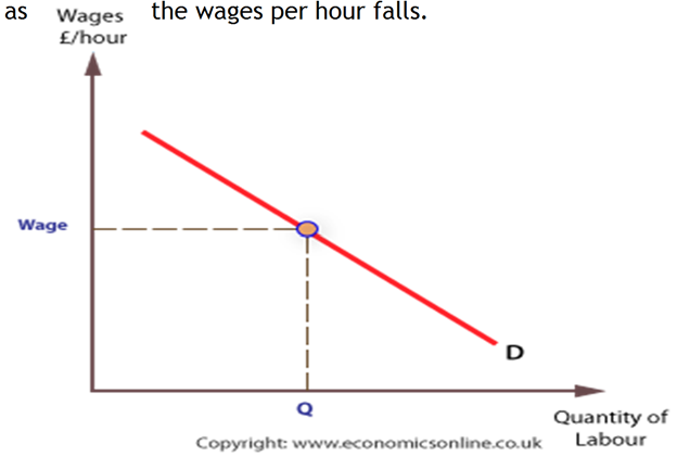\n\n * **Determinants of Labour Demand:** Consumer demand for final outputs; relative prices of capital equipment substitutes; marginal productivity of labour; and ancillary statutory employment expenses (e.g., pension contributions, employer insurance).\n\n* **The Supply of Labour:**\n * The total number of individuals willing and able to offer their labour at various wage rates.\n * The supply curve is upward-sloping: higher wage rates provide greater financial incentives for individuals to sacrifice leisure time for work.\n\n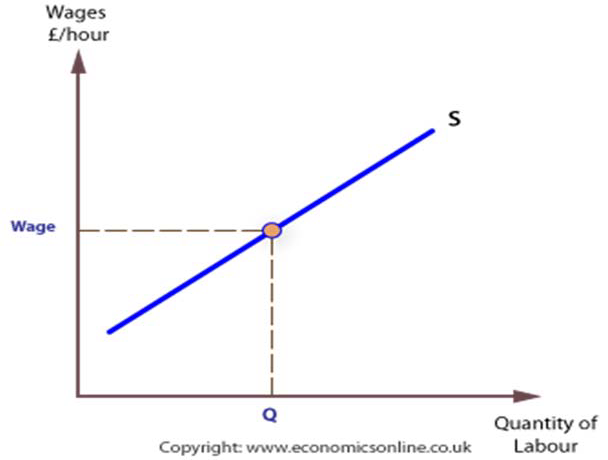\n\n * **Determinants of Labour Supply:** Total population size; net migration flows; population demographic age profile; statutory retirement age laws; compulsory schooling leaving ages; female labour participation rates; educational and vocational achievement levels; and geographic and occupational labour mobility.\n\n* **Shifts in Labour Equilibrium:**\n * **Shifts in Demand:** An increase in the demand for consumer goods (e.g., caps) shifts derived labour demand rightward from D$to$D_1$, raising the equilibrium wage rate from$W$to$W_1$and expanding employment from$Q$to$Q_1.\n\n\n\n* **Shifts in Supply:** An influx of qualified university graduates shifts labour supply rightward from S_1$to$S_2$, reducing the equilibrium wage rate from$W_1$to$W_2$and expanding total employment from$Q_1$to$Q_2.\n\n\n\n### Trade Unions and Government Regulation in Labour Markets\n\n* **Trade Union Operations:**\n * **Trade Union:** An association of employees formed to negotiate collectively with employers to secure improvements in compensation, safety provisions, and working conditions.\n * **Secondary Picketing:** Industrial strike actions carried out by union members at a firm or location distinct from their direct employer to support striking workers elsewhere.\n * **Closed Shop:** An employment arrangement requiring all workers within a firm to hold mandatory union membership.\n * **Wage Determination Impact:** Unions leverage collective bargaining power to set a wage floor (W_2$) above the comp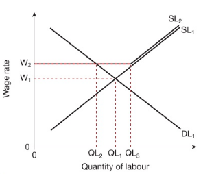etitive market equilibrium ($W_1$). Consequently, the effective labour supply curve becomes perfectly horizontal at$W_2$up to the original supply boundary ($QL_3$), reducing total employment demand to$QL_2.\n\n\n\n* **Consumer Protection and Market Competition Legislation:**\n * **Sale of Goods Act 1979:** UK statute stipulating that goods sold by businesses must be of merchantable quality and fit for their intended purpose (e.g., exterior house paint must not peel after one month of sun exposure; waterproof coats must prevent rain penetration).\n * **Food Safety Act 1990:** UK statute mandating that food products must comply with safety standards and be fit for human consumption (e.g., businesses are prohibited from selling previously defrosted and refrozen food or decaying fresh produce).\n * **Anti-Monopoly Regulation:** Public oversight to prevent anti-competitive mergers and abuse of market power, protecting consumers against excessive pricing, low quality, and restricted choice.\n\n* **Statutory Minimum Wage Legislation:**\n * A legally mandated wage floor set above the competitive market equilibrium wage, prohibiting employers from compensating workers below this hourly rate.\n * **Aims:** Safeguarding vulnerable workers against low pay, reducing income inequality, encouraging workforce participation, and reducing social welfare spending.\n\n| Socioeconomic Advantages | Socioeconomic Disadvantages |\n| :--- | :--- |\n| Enhances worker productivity and motivation. | Elevates employer operational wage costs. |\n| Increases financial incentives to seek employment. | Can cause classical unemployment if firms cut jobs. |\n| Alleviates absolute working poverty. | Induces cost-push inflation via passed-on consumer prices. |\n| Lowers government welfare claims. | Distorts competitive labour market clearing. |\n\n* **Graphical Analysis of Minimum Wage:**\n * Imposing a minimum wage (W_1$) above the equ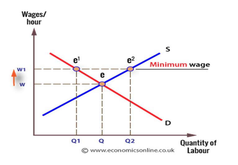ilibrium wage ($W$) reduces firm demand for labour to$Q_1$while expanding labour supply to$Q_2$, creating an excess supply of labour (unemployment gap equal to$Q_2 - Q_1).\n\n\n\n---\n\n# Unit 3: Government and the Economy\n\n### Macroeconomic Objectives and the Economic Cycle\n\n* **Foundational Macroeconomic Metrics:**\n * **Macroeconomics:** The branch of economic analysis dedicated to studying economy-wide aggregates, including national income, inflation, unemployment, and trade balances.\n * **Gross Domestic Product (GDP):** The total monetary value of all finished goods and services produced within an economy over a specific time period, excluding intermediate inputs to prevent double-counting.\n * **National Income:** The aggregate monetary earnings accrued by all factors of production within an economy over a financial year.\n * **The Economic Cycle:** Periodic fluctuations in national economic activity characterized by sequential phases of expansion, peak, contraction, and recovery.\n * **Unsustainable Economic Growth:** Rapid economic expansion achieved through the excessive consumption of finite natural resources, causing ecological degradation and compromising the living standards of future generations.\n\n* **The Four Phases of the Economic Cycle:**\n * **Boom / Peak (Red):** Maximum capacity utilization, high GDP growth rates, high employment levels, and accelerating demand-pull inflation.\n * **Downturn / Recession (Yellow):** Decelerating GDP growth, falling consumer and business investment, rising unemployment, and declining price inflation.\n * **Depression / Trough (Purple):** Extended contraction where real GDP falls sharply, plant capacity sits idle, unemployment reaches high levels, and prices drop.\n * **Recovery / Upturn (Green):** Resumption of positive economic growth, rising consumer confidence, expanding industrial production, falling unemployment, and firming price levels.\n\n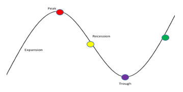\n\n* **Cyclical Fluctuations Table:**\n\n| Macroeconomic Factor | Boom Phase | Downturn Phase | Depression / Slump | Recovery Phase |\n| :--- | :--- | :--- | :--- | :--- |\n| **GDP Growth** | High and accelerating. | Growing at a slower rate. | Real GDP falls sharply. | Output begins to rise. |\n| **Employment** | High; labour shortages. | Unemployment begins to rise. | Unemployment increases sharply. | Unemployment begins to fall. |\n| **Inflation Rate** | High, increasing prices. | Inflation rate moderates. | Prices fall sharply (deflation). | Prices begin to rise gently. |\n\n* **Limitations of GDP as a Measure of Living Standards:**\n * **Price Inflation Distortions:** Unadjusted nominal GDP increases can reflect rising price levels rather than real expansions in output.\n * **Accounting Divergences:** Cross-national variations in data collection methods and accounting frameworks distort international comparisons.\n * **Home-Produced / Subsistence Output:** Non-monetized economic activity (e.g., subsistence farming, domestic caregiving) is excluded from official GDP tallies.\n * **Population Size Adjustments:** Aggregate GDP can expand while GDP per capita contracts if population growth outpaces output growth.\n * **External Costs:** Official GDP metrics treat production output positively while ignoring negative externalities such as industrial pollution and health risks.\n * **The Hidden / Informal Economy:** Unregistered transactions, cash-in-hand work, and black-market activities escape official tax recording.\n * **Leisure Time and Quality of Life:** GDP accounts fail to reflect working hours, personal leisure time, human rights, or societal well-being.\n\n### Inflation and Deflation\n\n* **Definitions and Measurement:**\n * **Inflation:** A sustained, generalized increase in the overall price level of goods and services in an economy, eroding currency purchasing power.\n * **Deflation:** A sustained, generalized decline in the average price level across an economy.\n * **Consumer Price Index (CPI):** A measure tracking average household living costs via a weighted basket of consumer goods and services, excluding housing costs like council taxes.\n * **Retail Price Index (RPI):** A broader measure tracking the average price level of a weighted basket that includes housing costs, mortgage interest payments, and local property taxes.\n * **Target Range:** Most central banks target an annual inflation rate of approximately `2\%$` to `$4\%$` (specifically `$2\%` in the UK) to support growth while avoiding deflationary spirals.\n\n* **Primary Causes of Inflation:**\n * **Demand-Pull Inflation:** Triggered when aggregate demand (AD$) outpaces aggregate supply ($AS) near full employment, pulling up price levels.\n * **Cost-Push Inflation:** Triggered when rising input costs (e.g., imported raw materials, energy shocks, wage increases, indirect taxes) compress profit margins, prompting firms to raise consumer prices.\n\n* **Macroeconomic Impacts of Inflation:**\n * **Purchasing Power:** Accelerating price levels diminish the real volume of goods and services purchasable per unit of currency.\n * **Wage-Price Spirals:** Rising living costs lead workers to demand higher nominal wages, raising firm operating costs and feeding further inflation.\n * **International Competitiveness:** Domestic inflation rates exceeding those of trading partners make exports more expensive and imports cheaper, worsening the current account balance.\n * **Menu Costs:** The administrative expense incurred by firms to recalculate and reprint menus, price lists, barcodes, and marketing displays.\n * **Shoe-Leather Costs:** The opportunity cost of time spent by consumers seeking competitive prices or moving funds to maximize deposit yields.\n * **Business Uncertainty and Investment:** Unpredictable inflation rates obscure expected rates of return, leading firms to delay long-term capital investments.\n\n### Unemployment\n\n* **Definition and Criteria:**\n * **Unemployment:** The condition of individuals within the active labour force who are capable of working and actively seeking work, but unable to secure paid employment.\n * **International Labour Organization (ILO) Criteria:**\n * Without a job, wanting a job, having actively sought employment within the previous `4\,\text{weeks}$`, and available to start work within the subsequent `$2\,\text{weeks}`; or\n * Out of work, having secured an employment contract, and waiting to take up the post within the subsequent `2\,\text{weeks}`.\n\n* **Five Structural Classifications of Unemployment:**\n * **Cyclical (Demand-Deficient) Unemployment:** Occurs during economic downturns and recessions when falling aggregate demand leads firms to reduce output and lay off workers.\n * **Structural Unemployment:** Caused by structural shifts in an economy, driven by:\n * *Geographical Immobility:* Inability of displaced workers to relocate to regions with active job vacancies due to housing costs or social ties.\n * *Technological Unemployment:* Capital equipment and digital automation permanently replacing manual and repetitive jobs.\n * *Sectoral Decline:* Long-term contraction of sunset industries (e.g., coal mining) leaving specialized workers with obsolete skill sets.\n * **Seasonal Unemployment:** Predictable fluctuations in labour demand tied to specific times of the year (e.g., tourism, agricultural harvesting).\n * **Voluntary Unemployment:** Individuals choosing not to participate in the active workforce at prevailing market wages, opting for state welfare or non-work activities.\n * **Frictional Unemployment:** Transitional unemployment experienced when individuals voluntarily leave one job to search for another, representing a functional job-matching process.\n\n* **Consequences of Unemployment:**\n * **National Output and GDP:** Idled labour resources place production inside the PPC, reducing actual GDP output below its potential.\n * **Public Finances:** Decreased tax revenues (income tax, VAT) paired with increased public spending on welfare benefits worsens budget deficits.\n * **Living Standards and Poverty:** Long-term joblessness depletes household savings, increasing poverty, personal debt, and home repossessions.\n * **Societal and Psychological Costs:** Extended unemployment is linked to family breakdown, declining life expectancy, and higher street crime.\n\n### The Balance of Payments Current Account\n\n* **Components of the Balance of Payments:**\n * **Balance of Payments:** A financial record tracking all economic transactions between domestic residents and the rest of the world over a specified time period.\n * **Current Account Components:**\n * *Trade in Goods (Visible Trade):* Net balance of exports and imports of tangible, physical products (e.g., cars, oil, machinery).\n * *Trade in Services (Invisible Trade):* Net balance of exports and imports of non-tangible services (e.g., international tourism, insurance, banking).\n * *Primary Income:* Cross-border earnings flows from factor inputs abroad, including employee compensation, investment dividends, and loan interest payments.\n * *Secondary Income:* Unilateral international transfers without reciprocal economic returns (e.g., international aid payments, government contributions to overseas bodies).\n\n* **Current Account Balances:**\n * **Current Account Deficit:** When total expenditures on imported goods, services, and net income transfers exceed gross export receipts.\n * **Current Account Surplus:** When gross export revenues and net income receipts exceed total expenditures on imports.\n * **Exchange Rate Conversion Example:**\n * At an exchange rate of `\$1 = £0.79$`, converting `$\$4` yields:\n\n\$4 \times £0.79 = £3.16\n\n* **Determinants of Current Account Balances:**\n * *Relative Quality of Goods:* Superior domestic engineering increases export volumes; superior foreign manufacturing increases import demand.\n * *Relative Price Levels:* Higher domestic inflation makes domestic goods uncompetitive, expanding imports and contracting exports.\n * *Real Exchange Rate Movements:* Currency depreciation lowers foreign-currency export prices while raising domestic-currency import prices, improving the current account balance.\n * *Domestic Income Levels:* Rising domestic real incomes increase consumer expenditure on imported luxury goods and overseas travel.\n\n### Income Inequality and Poverty\n\n* **Classifications of Poverty:**\n * **Absolute Poverty:** A severe condition where individual income is insufficient to secure basic human survival needs, including food, clean water, shelter, and sanitation.\n * **Relative Poverty:** A condition where household income falls significantly below the median average income of a nation, preventing participation in standard societal living norms.\n\n* **Drivers of Income Inequality:**\n * Unequal educational access and differences in technical skills, human capital, and natural aptitudes.\n * Wage disparities between high-skill knowledge professionals and manual workers.\n * Unequal ownership of inherited wealth, commercial property, and dividend-yielding equities.\n * Systemic joblessness, structural economic displacement, and regional underinvestment.\n\n* **Government Intervention Strategies:**\n * **Progressive Taxation:** Imposing higher marginal income tax rates on higher income brackets, using the revenues to narrow the income gap.\n * **Social Benefit Transfers:** Distributing targeted welfare payments (e.g., universal child benefits, unemployment stipends, disability grants) to support lower-income households.\n * **Public Investments in Education and Healthcare:** Providing state-funded schooling and universal healthcare ensures equal opportunities, improving human capital and upward socioeconomic mobility.\n\n### Fiscal Policy\n\n* **Mechanics of Fiscal Policy:**\n * **Fiscal Policy:** The manipulation of government spending (G$) and taxation ($T$) to influence the level of aggregate demand ($AD) and economic activity.\n * **Tax Classifications:**\n * *Direct Taxes:* Levies imposed on the income, wealth, or corporate profits of individuals and enterprises (e.g., income tax, corporation tax).\n * *Indirect Taxes:* Levies imposed on the expenditure and consumption of goods and services (e.g., VAT, ad valorem duties).\n * *Environmental Taxes:* Levies designed to penalize polluting activities and internalize negative externalities (e.g., landfill levies, carbon duties).\n * *Regressive Taxes:* Levies that extract a larger percentage of income from low-income earners than from high-income earners (e.g., flat indirect taxes).\n * **Fiscal Balances:**\n * *Fiscal Deficit:* Occurs when public spending exceeds tax revenues (G > T), requiring the state to issue sovereign debt.\n * *Fiscal Surplus:* Occurs when tax revenues exceed government expenditures (T > G), enabling sovereign debt repayments.\n\n* **Stances of Fiscal Policy:**\n * **Expansionary Fiscal Policy:** Involves reducing taxes and increasing government spending (G \uparrow, T \downarrow) to stimulate aggregate demand, accelerate GDP growth, and reduce cyclical unemployment.\n * **Contractionary Fiscal Policy:** Involves raising taxes and trimming public expenditures (G \downarrow, T \uparrow) to dampen aggregate demand, curb demand-pull inflation, and narrow current account deficits.\n\n### Monetary Policy\n\n* **Mechanics of Monetary Policy:**\n * **Monetary Policy:** Central bank actions adjusting benchmark interest rates and the domestic money supply to influence macroeconomic activity.\n * **Functions of Central Banks:** Formulating monetary policy; achieving statutory inflation targets; acting as banker to the government; regulating commercial banks; acting as lender of last resort; and managing official foreign currency reserves.\n * **Monetary Policy Committee (MPC):** In the UK, a committee of nine economic experts that sets benchmark policy interest rates, evaluating metrics including GDP growth, inflation, and unemployment.\n\n* **Macroeconomic Impacts of Benchmark Interest Rate Cuts:**\n * Reduces the cost of commercial borrowing, encouraging firms to finance capital investments.\n * Lowers residential mortgage payments, increasing household disposable income.\n * Diminishes financial incentives to save, spurring consumer expenditure.\n * Triggers capital outflows and depreciates the domestic currency, lowering foreign-currency export prices and boosting net export demand.\n * *Policy Risk:* Excessive monetary expansion can overheat the economy, fueling demand-pull inflation.\n\n* **Quantitative Easing (QE):**\n * An unconventional monetary intervention used when nominal policy rates approach the zero-lower bound:\n * Step 1: The central bank determines the financial injection required to stimulate aggregate demand.\n * Step 2: The central bank generates digital central bank reserves.\n * Step 3: These funds are used to purchase government bonds from commercial banks and institutional investors.\n * Step 4: Asset purchases inject liquidity into the commercial banking sector, lowering long-term bond yields.\n * Step 5: Commercial banks expand lending to businesses and households at lower interest rates.\n * Step 6: Broad credit expansion stimulates consumer spending and corporate capital investment, aiding recovery from recession.\n\n### Supply-Side Policies\n\n* **Foundational Supply-Side Objectives:**\n * **Supply-Side Policies:** Microeconomic interventions designed to shift the aggregate supply curve (AS) rightward by expanding productive capacity, elevating factor productivity, and removing market rigidities.\n\n* **Key Supply-Side Policy Interventions:**\n * **Education and Vocational Training:** Upgrading the skills of the national workforce improves labor productivity, encourages technological adoption, and reduces structural unemployment.\n * **Corporate Deregulation:** Removing administrative red tape and lowering business licensing costs encourages entrepreneurial startups and enhances market competition.\n * **Privatization:** Exposing previously nationalized public utilities to commercial market disciplines incentivizes operational efficiency and cost reductions.\n * **Labour Market Reforms:** Limiting trade union disruption and reforming minimum wage constraints reduces firm hiring expenses and increases operational flexibility.\n * **Tax Relief:** Lowering corporation tax rates increases expected returns on capital investments, while reducing marginal income tax rates strengthens incentives to work.\n * **Infrastructure Spending:** Upgrading transport corridors, electrical power grids, and digital communication networks lowers logistics and distribution expenses across the economy.\n\n### Policy Conflicts and Trade-Offs\n\n* **Structural Macroeconomic Trade-Offs:**\n * **Inflation vs. Unemployment (Short-Run Phillips Curve Trade-Off):** Lowering interest rates to stimulate output and reduce unemployment can overheat the economy and generate demand-pull inflation. Conversely, raising interest rates to curb inflation can prompt firms to cut jobs.\n * **Economic Growth vs. Environmental Protection:** Accelerating GDP expansion often drives the depletion of non-renewable fossil fuels and raises industrial emissions. Sustainable practices, meanwhile, can raise business operating costs and slow growth.\n * **Inflation vs. Current Account Balance:** Raising domestic interest rates to contain inflation can attract foreign capital inflows, appreciating the currency. This makes exports more expensive and imports cheaper, worsening a current account deficit.\n * **Economic Growth vs. Income Inequality:** Pro-growth supply-side policies (e.g., cutting top marginal tax rates, deregulating labor markets) often widen the income gap between wealthy capital owners and low-skill workers.\n * **Economic Growth vs. Demand Inflation:** Rapid expansion in aggregate demand without corresponding investments in productive capacity generates resource bottlenecks, driving up price levels.\n\n* **Policy Solutions for Macroeconomic Trade-Offs:**\n * *Inflation vs. Unemployment:* Combine monetary discipline with supply-side workforce retraining and targeted regional subsidies.\n * *Growth vs. Environment:* Offer green technology subsidies and trade relief to firms adopting renewable power systems.\n * *Growth vs. Income Inequality:* Use progressive taxation alongside public investments in health and educational access for low-income households.\n\n---\n\n# Unit 4: The Global Economy\n\n### Globalization and Multinational Corporations (MNCs)\n\n* **Foundations of Globalization:**\n * **Globalization:** The deepening economic integration and interdependence among national economies worldwide.\n * **Defining Characteristics:** Cross-border trade in goods and services; free international capital and investment flows; migration of labor; cross-border transfers of technological intellectual property; and economic interdependence among nations.\n * **Key Drivers of Globalization:**\n * Progressive reduction of tariffs and import quotas via multilateral trade negotiations.\n * Reductions in sea, rail, and air freight costs due to innovations like shipping containerization.\n * Reductions in international telecommunication expenses via high-speed internet infrastructure.\n * Commercial expansion of Multinational Corporations (MNCs) establishing cross-border supply chains.\n\n* **Multinational Corporations (MNCs) and Foreign Direct Investment (FDI):**\n * **Multinational Corporation (MNC):** A commercial enterprise headquartered in one country that manages operational production facilities across other host countries.\n * **Foreign Direct Investment (FDI):** Capital investments made by a foreign firm to acquire lasting operational control or establish new production facilities within a host country.\n\n* **Socioeconomic Impacts of MNCs on Host Economies:**\n * **Positive Impacts:** Large-scale job creation; capital-deepening through modern factories; technology and skills transfer to domestic suppliers; infrastructure upgrades; and expanded tax revenues.\n * **Negative Impacts:** Repatriation of operating profits back to headquarters; tax avoidance strategies (e.g., transfer pricing); displacement of domestic enterprises; environmental degradation; and worker exploitation in weakly regulated host nations.\n\n### International Trade, Specialization, and Free Trade\n\n* **Rationale for International Trade:**\n * **Acquiring Non-Domestic Resources:** Allows countries to obtain resources unavailable domestically (e.g., petroleum, agricultural commodities, industrial minerals).\n * **Exploiting Comparative Efficiencies:** Enables countries to purchase goods produced overseas at lower opportunity costs due to specialized regional production.\n * **Exporting Surplus Commodities:** Allows nations with abundant natural resources to sell excess output in global markets, raising national income.\n\n* **Economic Benefits of Free International Trade:**\n * Consumers benefit from lower prices, greater choice, and higher-quality imported goods.\n * Domestic firms secure lower-cost intermediate components and raw materials, enhancing competitiveness.\n * Exporters access broader global markets, enabling them to exploit economies of scale.\n\n* **Economic Risks of Unregulated Free Trade:**\n * Domestic manufacturing firms face competition from low-wage overseas producers, risking industrial closures.\n * Vulnerability to structural and technological unemployment within displaced domestic manufacturing sectors.\n * Exposure to global economic disruptions and financial crises.\n\n### Trade Protectionism\n\n* **Definitions and Instruments:**\n * **Protectionism:** The implementation of government policy measures to protect domestic producers from foreign competition and restrict imports.\n * **Tariffs (Customs Duties):** Indirect excise taxes levied on imports to raise their domestic price, reducing foreign demand and encouraging domestic consumption.\n * **Quotas:** Physical limits on the volume of a specific good permitted into an economy over a set period.\n * **Production Subsidies:** Direct government grants provided to domestic firms, lowering their production costs and allowing them to price output competitively against imports.\n * **Dumping:** The unfair trade practice where overseas firms sell large export volumes below their domestic market price or below production cost to drive out domestic rivals.\n\n* **Strategic Motivations for Trade Protectionism:**\n * Defending domestic infant industries until they establish economies of scale.\n * Protecting domestic jobs against low-cost overseas labor.\n * Preventing foreign exporters from dumping predatory surpluses.\n * Generating fiscal tariff revenues for the government.\n * Halting imports of harmful or dangerous products (e.g., illicit narcotics, substandard food).\n * Retaliating against discriminatory trade barriers imposed by foreign trading partners.\n * Correcting persistent current account balance deficits.\n\n* **Graphical Analysis of Protectionist Instruments:**\n * **Tariffs and Quotas:** These measures restrict the market supply of foreign imports, shifting the total market supply curve leftward from S_1$to$S_2$. Conseque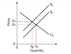ntly, the domestic market price rises from$p_1$to$p_2$while quantity falls from$q_1$to$q_2.\n\n\n\n* **Domestic Subsidies:** Granting financial subsidies lowers the production costs of domestic firms, shifting total market supply rightward from S_1$to$S_2$. This redu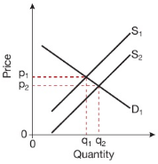ces domestic market price from$p_1$to$p_2$and expands market quantity from$q_1$to$q_2.\n\n\n\n### Trading Blocs and Multilateral Trade Agreements\n\n* **Hierarchy of Regional Trading Blocs:**\n * **Preferential Trade Areas (PTAs):** Agreements where partner nations reduce tariffs on selected goods while maintaining trade barriers on others.\n * **Free Trade Areas (FTAs):** Complete elimination of tariffs and quotas on trade between members, while each nation maintains its own independent trade barriers against non-member countries (e.g., NAFTA / USMCA).\n * **Customs Unions:** Elimination of internal trade barriers alongside the adoption of a Common External Tariff (CET) applied to non-member nations (e.g., Southern African Customs Union - SACU).\n * **Common Markets:** Customs unions that also eliminate restrictions on the free movement of labour, capital, and enterprise between member countries.\n * **Economic Unions:** Common markets featuring deep integration, including harmonized fiscal regulations and common monetary policy (e.g., the European Union).\n\n* **Economic Impacts of Trading Blocs:**\n * **Advantages for Members:** Cheaper imported consumer goods; expanded market scale; trade-creation efficiencies; increased FDI; and reduced regional geopolitical conflict.\n * **Disadvantages for Members:** Trade diversion away from more efficient low-cost non-member producers; loss of independent trade policy; and vulnerability to regional economic shocks.\n\n* **Prominent Global Trading Blocs:**\n * **NAFTA / USMCA:** Commercial free trade area linking the United States, Canada, and Mexico.\n * **ASEAN:** Association of Southeast Asian Nations, a 10-member bloc including Thailand, Malaysia, Singapore, and regional partners.\n * **SACU:** Southern African Customs Union, uniting Botswana, Namibia, South Africa, and regional neighbors.\n\n### The World Trade Organization (WTO)\n\n* **Role of the WTO:**\n * **The World Trade Organization (WTO):** An international regulatory organization that oversees global trade agreements, resolves cross-border trade disputes, and encourages trade liberalization.\n * **Core Functions:** Mediating multilateral trade negotiations; monitoring member adherence to global trade agreements; settling bilateral trade disputes; and integrating developing nations into global trade systems.\n\n* **Criticisms of the WTO:**\n * Undemocratic governance that often prioritizes corporate commercial interests over national labor and environmental protections.\n * Permitting rules that exploit working standards in developing nations.\n * Overturning domestic environmental protection policies that conflict with free trade rules.\n * Institutional bias favoring developed nations, occasionally marginalizing low-income developing nations in negotiations.\n\n* **Global Trade Patterns:**\n * **Developed Economies:** Long-term transition from traditional manufacturing toward knowledge-intensive tertiary services; expansion of international budget air travel; and persistent internal income inequality.\n * **Developing Economies:** High net outward migration flows; growing FDI inflows (notably across the African continent); reliance on primary commodity exports; and pursuit of multilateral debt relief and WTO trade barrier reductions.\n\n### Exchange Rate Determination and Currency Fluctuations\n\n* **Exchange Rate Concepts:**\n * **Exchange Rate:** The price of one national currency expressed in terms of another.\n * **Floating Exchange Rate:** A regime where currency valuations are determined freely by market supply and demand within foreign exchange markets.\n * **Appreciation:** An increase in the market value of a floating currency relative to another currency.\n * **Depreciation:** A decrease in the market value of a floating currency relative to another currency.\n * **Revaluation:** An explicit, deliberate upward adjustment of a pegged currency value by the government or central bank.\n * **Devaluation:** An explicit, deliberate downward adjustment of a pegged currency value by the government or central bank.\n\n* **Determination of Floating Exchange Rates:**\n * Floating exchange rates clear at the intersection of currency market demand and supply curves.\n * *Example:* The equilibrium exchange rate of the British Pound clears at `£1 = \$1.50$` at quantity$Q.\n\n\n\n* **Factors Affecting Currency Demand and Supply:**\n * **Determinants of Currency Demand:** Inflows of foreign capital into domestic banks driven by high domestic interest rates; foreign currency speculation anticipating currency gains; growing overseas demand for exports; and foreign multinational direct investments.\n * **Determinants of Currency Supply:** Domestic residents purchasing foreign assets to chase higher overseas interest rates; speculative selling anticipating currency depreciation; and domestic demand for imports requiring the conversion of local currency into foreign funds.\n\n* **Market Shifts in Currency Exchange Rates:**\n * **Increase in Currency Supply (Depreciation):** An expansion in the supply of Australian Dollars from S_1$to$S_2$(driven by rising domestic demand for imports) lowers the exchange rate from$P$to$P_1$while expanding transacted quantity from$Q_1$to$Q_2.\n\n\n\n* **Increase in Currency Demand (Appreciation):** An expansion in the demand for British Pounds from D$to$D_1$(driven by rising overseas demand for UK exports) raises the exchange rate from `$£1 = \$1.50$` to `$£1 = \$1.60$` while expanding transacted volume from$Q$to$Q_1.\n\n\n\n* **Macroeconomic Impacts of Currency Movements:**\n * **Impact of Depreciation (e.g., Pound drops from `£1 = \$1.50$` to `$£1 = \$1.20`):**\n * *Exports:* Become cheaper in foreign currencies, stimulating export demand.\n * *Imports:* Become more expensive in domestic currency, dampening import volumes.\n * *Current Account:* The trade balance improves, provided the Marshall-Lerner condition holds (elastic export and import demand).\n * **Impact of Appreciation (e.g., Pound rises from ` £1 = \$1.20$` to `$£1 = \$1.50$$`):** * Exports: Become more expensive abroad, reducing foreign export demand. * Imports: Become cheaper domestically, expanding import expenditures. * Current Account: The current account balance worsens, expanding deficits.

• Policy Limitations: Central banks can influence exchange rates by adjusting interest rates (since interest rates and exchange rates are directly related). However, lowering rates to weaken a currency can generate domestic inflation and conflict with other macroeconomic policy goals.