AP Calculus AB Ultimate Guide
Unit 1 - Limits and Continuity
A limit is the intended height of a graph, as x gets very close to a value. This means that when we follow a function, the limit will show what the height that the point is supposed to be, even if it doesn’t concur with the actual function
Take this limit for example →
We can find this limit by plugging in x to the function → 4 + 10 + 6 / 4 → 5
Solving Limits
When you substitute the number and get , there are a few different ways you can solve it.
Factoring and eliminating the hole →
The first option is factor the function so that we can eliminate the hole →
Then, once you eliminate the hole, plug the value in again→
Making 1 fraction →
First, to get the numerator sorted out, we need to find a common denominator for the two fractions in the numerator →
Now, we can simplify the fraction to get one fraction →
Multiplying by conjugate →
In this situation, it would be best to try multiplying by the conjugate →
When we multiply everything out, we know that we only have to do the front terms and the back terms so we get →
Here are some rules for limits as well! You can use these to help assist you in solving limits:
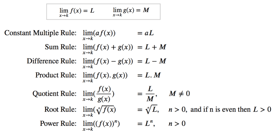
It is also helpful to remember →
x can be any number or symbol, but when it is the same on the bottom and top, it is equal to 1
I’ve also seen this limit rule →
Finding Limits Graphically / Numerically
Another way to find limits is by looking at a graph.
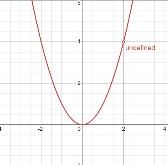
For a limit to exist, the function must approach the same height value from both sides
In this example, the limit does exist even though there is a hole because the function approaches the same height from both sides
When the function approaches two different heights, the function might have an actual value, but the limit does not exist (mean girls reference!)
Here is an example, where the f(2) = 4, but the limit DNE
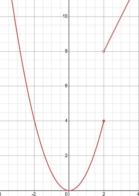
Limits approaching from the left side will have a - sign above the number (like 2-) and limits approaching from the right has a + sign above the number (like 2+)
We can also find limits from the table
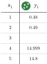
Don’t pay attention to the number it is approaching, as both sides may be approaching something different. In this example we can see that → and
Because both limits approach something different, the limit does not exist →
Squeeze Theorem
if g(x) <= f(x) <= h(x), while x does not equal c, in some interval about c, and , then
Basically, the function f(x) is in between two functions (g(x) <= f(x) <= h(x)). By taking the limit of each function, and solving it, we can get the value of f(x).
When g(x) and h(x) are different, the limit of f(x) cannot be determined
Vertical Asymptotes
A vertical asymptote is defined as → the line x = a is a vertical asymptote of the graph of a function f(x) if either
If you get confused with horizontal, remember that vertical asymptote limits will be approaching a NUMBER and result in ±infinity
You can find them by looking at a graph or looking at a table. The table will have values that get really big (in either pos or neg direction) really fast
You can find them without a calculator however
When direct substitution gives you , you know it’s a vertical asymptote
The only possible one-sided limits are +∞ or -∞
Pick a value just to the left or right of your x on the side you are approaching from, and consider whether your height is positive or negative. This will give you the sign of the limit
Example →
Horizontal Asymptotes
A horizontal asymptote is defined as → the line y = b is a horizontal asymptote of a function f(x) if either
If you get confused with VA, remember that hortizontal asymptote limits will be approaching infinity and give 0/NA/#
It is also helpful to remember BOBO BOTNA EATSDC (Bigger On Bottom = 0; Bigger On Top = No Asymptote; Exponents Are The Same = Divide Coefficients)
You can also find these by looking at a graph, but with horizontal asymptotes it takes some mental imagining (example function →
First, find the end behavior for the function, so just cancel out anything that isn’t the highest degree →
Next, we need to think about both limits, so taking the limit of the end behavior as x approaches ± ∞.
If the denominator grows faster than the numerator, it gets smaller and smaller towards 0
If the numerator grows faster than the denominator, then the function will grow towards ± ∞, and therefore no HA
If the exponents are the same, then the limits will both approach the divided coefficients
In our case, 3/5x, the 5x will continue to grow further, while the numerator stays the same, meaning that the fraction will get closer and closer to 0
Continuity
Here are the types of discontinuity in graph form →
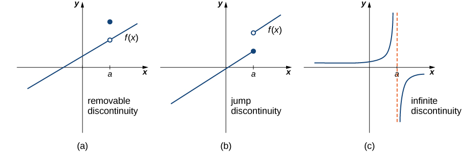
Removable
The limits approaching the left or the right are equal, but the actual value is not
Jump
Here, the limits do not match, the function value may be the same as one of the limits, however
Infinite
Here, the actual value does not exist and the limits approach infinity
Expanding the function to be continuous
When a function has a removable discontinuity, it is sometimes possible to extend the function. To do this, find the discontinuity and simply add the term to the existing piece wise function
Making functions continuous
Since a continuous function is , we can use this in the following problem
x=4 would be the actual value, and the other one would be the limit as x approaches 4. This means we just have to set them equal to each other and set x=4, meaning that we end up with 6 = k² - 2 →k = 2
Intermediate Value Theorem (IVT)
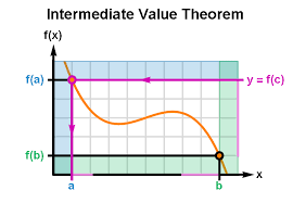
The IVT explains if a function is continuous between a and b, then it will pass through every value between f(a) and f(b)
for example, if we have the points (1, -1) and (2, 5) and we want to know about any real solutions where f(x) = x3 - x - 1. Here is how to justify →
check for continuity → f(x) is continuous, so IVT applies
sandwich your values → f(1) = -1 < 0 < 5 = f(2)
Answer (yes/no) by IVT → There is a real solution by IVT
Unit 2 - Differentiation: Definition and Fundamental Properties
Remember our average rate of change formula →
But… what if we want to find the slope at one point? Finding that using our formula would lead to a number over zero
let’s say we have a function x². If we want the slope at point x=2, we take another point, for example (3, 9), and move that point closer and closer to x=2 until it gets infinitely close, and take the slope of that
That gives us the definition of a derivative
The definition of a derivative is this →
Basically it is , except we want to find the instantaneous rate of change (the rate of change of a single point). By differentiating a function, we get the derivative which is the rate of change at each point on a function
For example, find
, now time to cancel terms!
This fits within the power rule! Because →
Higher Order Notation
Let’s say we have the function f(x) = cos(x).
Finding the derivative of the derivative would be called the second derivative and would be written as so →
Higher order derivative is noted by adding more primes or by this notation →
Alternative Definition of Derivative
You might also see the derivative written these ways
In these cases, a is a plugged in value. You won’t have to manually solve these limits, but there is 3 things you should do
1 - find/spot the original function
2 - find the derivative of that function
3 - plug in any points (a) if you have to
Derivative Rules
Here are some more derivative rules:
Constant Rule →
Coefficients →
Addition/Subtraction →
Power Rule →
Product Rule →
You can remember this rule by simply remembering that it’s just multiplying by each others derivatives
If there is three or more terms, you do it like so →
Quotient Rule →
A way to remember this rule is that double ds come first (denominator x derivative) and then you switch (numerator x derivative). And then you just have to bring the denominator over and square it!2
Another way to remember this is “low d high - high d low over low squared”
You also sometimes might be able to work out problems without the quotient rule like so →
Tangent & Normal Lines
A tangent line is the line at that point tangent to the function. To find the tangent line, you will need to use point slope formula (y2 - y1 = m(x2 - x1)), but instead of m, we plug in the slope from the derivative
For example, find the tangent line at point x=2 for the function f(x) = 2x²
First, we need to plug in the point to the original function f(2) = 8
Then, find the derivative of f →f’(x) = 4x
Then, we need to plug in 2 in the derivative → f’(2) = 8
Then using these values, we get the tangent line equation →
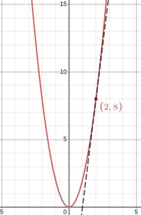
The slope for a normal line is just perpendicular, so the normal line equation would be → y - 8 = (-1/8)(x-2)
Linear Approximation
linear approximation is using a tangent line to approximate a value
Example, we want the value of x = 8.1 when y = √x
First, we write a tangent line close to the point, at x = 8
Now that we have slope, the y-coordinate of the point would be √8, so our tangent line would be →
Using this tangent line, we can plug in the real value of x, 8.1, and get out our y-value →
That is very close to the actual value y(8.1)!
Points Parallel to Lines
At what point on the graph y = 3x + 1 is the tangent line parallel to the line y = 5x -1
We already know what slope we should be looking for and that is 5, because it is parallel, so we need to set the derivative equal to the slope →
Now, we need to solve for the x-value →
Now that we have our x-value, we can solve for the y value, by simply plugging that x-value back into our undifferentiated function →
That gives us our messy looking point
Differentiability
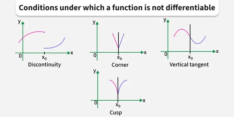
In order to be differentiable, a function must have equal one-sided derivatives and be continuous where the rule for the function changes
This means that → DIFFERENTIABILITY implies CONTINUITY
if f’(a) exists, then f(a) is continuous
However, the inverse is not true… just because something is continuous doesn’t imply differentiability
How to check if a piecewise function is differentiable
Given this piecewise function:
First, we need to check continuity
So, continuity is good!
Now, we need to check the derivatives →
Because our left and right derivatives are not equal, the function isn’t differentiable @ x=1 and f’(1) DNE. However, this function is still continuous
Derivatives of Trig Functions
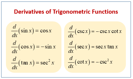
Ways to remember
the functions with c are always negative (cos=-sin, csc=-csccot, cot=-csc²)
sin loves cos, but cos doesn’t love sin (sin=cos, cos=-sin)
the tangents are always squared and love their partners more (sec², -csc²)
the sec and csc are self absorbed and always with their tangent partners (-csccot & sectan)
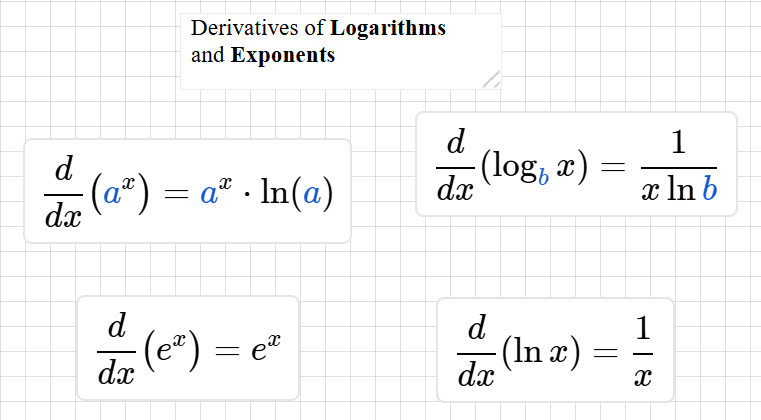
Derivatives of Exponents & Logarithms
Unit 3 - Differentiation: Composite, Implicit, and Inverse Functions
The Chain Rule →
The chain rule is used for functions inside of functions. It works like Russian nesting dolls the derivative of the outside function with all the normal dolls inside, then multiplied by the derivative of the next doll inside with the rest of the dolls inside
Example →
Implicit Differentiation
Sometimes, the functions aren’t always explicitly defined and we have both x and y → x² + y² = 1
Remember that taking the d/dx of x is just 1! Think of it like the chain rule → d/dx(f(x)) = f’(x) * 1. However, when we take the derivative of y with respect to x, that is dy/dx or y’.
This just means that whenever we are taking the derivative of y, we have to multiply it by dy/dx. A more complicated explanation is because of the chain rule, treating the singular function f(x) as a “f(g(x))” composite function, where the outside is “f( )” and inside is “x”
f’(x) * x’, but x’ (or dx/dx) is 1 so we normally leave it out, but with y →
This is why we have to multiply by dy/dx when taking the derivative of a non-x variable with respect to x
But you don’t really need to remember that, just remember that when taking the derivative of y, you have to multiply by dy/dx
Here is the steps to implicit differentiation
Differentiate both sides of the equation with respect to x
Collect the terms with dy/dx on one side of the equation. Any time you have to take the derivative of y, multiply by dy/dx
Factor out dy/dx and/or solve for dy/dx
Tangent Lines
Let’s say we wanted to find the tangent line to the curve of x² - xy + y² = 7 at the point (-1, 2)
We’re already given the point, so we just need to find the derivative. For this one, we have -xy so we use product rule (xy’ + yx’)
Now, we need to plug it into the derivative equation
Now, we can use this and the point to find the tangent and normal lines
Higher Order Derivatives
When we do higher order derivatives with implicit differentiation, we solve for the first derivative like normal, but whenever we start solving for the second one, we substitute dy/dx with our first derivative. Example → what is the second derivative of 5 = x² - cos(y)
Find the first derivative →
Then we need to use the quotient rule to find the second derivative (substituting dy/dx with our first derivative) →
Then, we can get rid of that numerator fraction by multiplying a sin(y) to the top and bottom →
Inverse Function Derivatives
An inverse function derivative is as so →
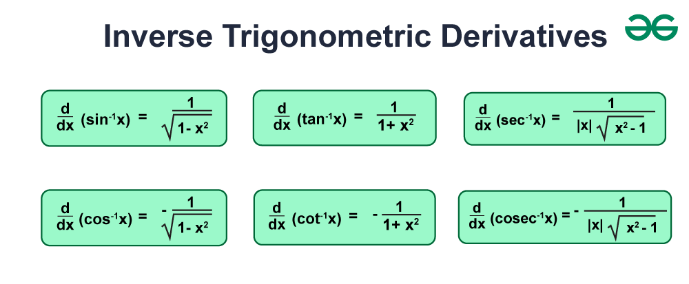
Ways to remember
Like our regular derivatives, the ones that start with c are always opposite to their partners
They are always 1 / something and always have an x²
You can think about it from easiest to hardest
Tangent and cotangent are easiest because it’s just 1 + x²
Sin and cos are next because they have sqrt and subtraction
Sec and csc are the most complicated and have | x |, sqrt, and flipped order, and subtraction
Unit 4 - Contextual Applications of Differentiation
Critical Points
To start, a critical point is any point where f’(x) = 0 or DNE. On the function f(x), they are all local extrema

In order for an x-value to be a critical point, that x-value must be in the domain of the function. So we need to look out for anything like
Dividing by 0
Taking the nth root of an even power
Taking the logarithm of 0 or a negative number
Example with function f(x) = x² / x - 1
Find domain of f(x) → x ≠ 1
Find the derivative →
Now, because we have an instance of dividing by 0, we can solve for when f’(x) = 0 or DNE (In this case, we can set the numerator = 0 to find when f’ = 0 and the denominator = 0 to find when f’ DNE). When we find these, we need to check back to our domain and see if the points are included
So our critical points are x = 0, 2
Example with piecewise function →
Our domains would be [0, 1] and [1, 4], however because we have 1 on both, we need to check for continuityd
Next, find when f’ = 0. Our f’ would consist of -2x-2 and -2x+6. So we just set them both to 0
, which is outside of the domain
Now to find when f’ does not exist. The only place where y’ might not exist is where those two functions meet (@ x = 1), so we check the one sided derivatives
, so, y’(1) DNE, meaning it is a critical point
Extreme Values
If f is continuous on a closed interval [a, b], then f has both a maximum and minimum value on the interval. These are either:
The values of f at the critical points in the open interval (a, b)
f(a) or f(b), the values of f at the endpoints
To find absolute extrema, we use the candidates test (basically a t-chart of the endpoints, and any critical points to find the highest and lowest values)
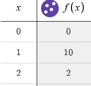
Example →
First, find the derivative →
Next, find the critical points →
Now, for the candidates test, we have our endpoints, 0 and 2, and then our critical points. Here we can see that our absolute max is 10 @ x=1, and our abs min is 0 @ x = 0
Intervals of Inc & Dec
When f is continuous and differentiable…
when f’ > 0, f is increasing
when f’ < 0, f is decreasing
The First Derivative Test determines if critical points are local mins, maxes, or neither
First find the critical points, then check for sign changes on f’
If f’ changes from + → -, then f has a maximum
If f’ changes from - → +, then f has a minimum
If f’ doesn’t change, then there is no local extreme
If there is endpoints, we need to consider the sign on f’ in the interval to the left/right of the endpoint and interpret whether f is increasing/decreasing approaching the endpoint to identify if it is a max or min
Example →
Our domain is continuous, so we don’t have to worry about it
Find the derivative →
Now, find the critical points →
Now that we have these points, we can perform the first derivative test. This is putting them on a number line and plugging in values in between the critical points to determine whether the sign is - or +
As we see here, our intervals of increasing would be and our intervals of decreasing would be
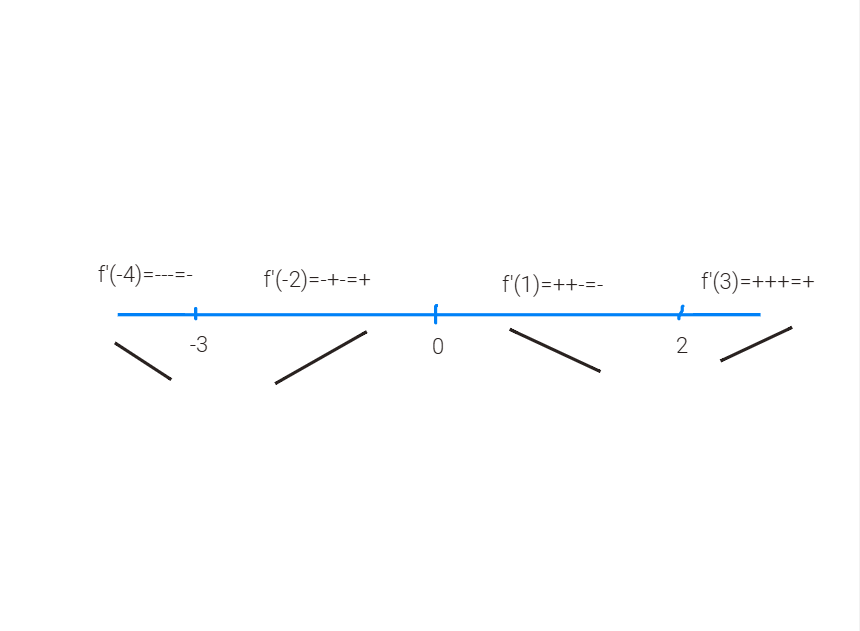
We can see that when both lines go down (switching from - → +), we have a local minimum. In this case it would be x = -3, 2
And when the lines both go up (switching from + → -), we have a local maximum. In this case it would be x = 0
Concavity and Inflection Points
Concavity is the curvature of the graph. For the concavity test, to find the signs of the second derivative, we use the second derivative instead of the first.
f is concave up when f’’ > 0
f is concave down when f’’ < 0
Points of inflection are where the concavity changes. In order to be a POI, it must be in the domain and change signs
Example →
Our domain is all real numbers, so no need to worry
We need to find our second derivative →
Now, setting it = 0, we get our potential points of inflection →
Now, like what we did before, we put this point on a number line and plug in values beside it to see whether it’s concave up/down and to see if the sign changes
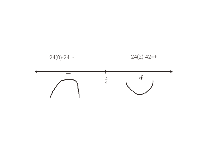
We can see that it’s concave down from (-infinity, 7/4) and concave up from (7/4, infinity)
Because the sign changes, there is an inflection point at x = 7/4
The Second Derivative Test is that by finding the sign of the second derivative at a critical point, we can determine whether the critical point is a maximum or a minimum
if f’ = 0 and f’’ < 0, then f has a local maximum
if f’ = 0 and f’’ > 0, then f' has a local minimum
Example →
Find second derivative →
Now, we plug in the critical points to see what the sign is → 6(2) = +, 6(-2) = -
This means that x = 2 is a local min and x = -2 is a local max
Mean Value Theorem
Remember that differentiability implies continuity!
The Mean Value Theorem for derivatives states that if f(x) is continuous at every point of the closed interval [a, b] and differentiable at every point of it’s interior (a, b), then there is at least one point c in (a, b) at which the derivative = average ROC of a & b or

Again, two conditions need to be met for this:
f(x) is continuous on [a, b] → to verify this, check any dividing by 0, sqrt of neg numbers, or logs of neg #s or 0
f’(x) is differentiable on (a, b) → to verify this, check the same as continuity but on the derivative
Example → y = x² on [0, 2]
First, check if y is continuous. There is no cases where we’d / 0, have sqrts of negative numbers, or logs of negative numbers, so it is continuous
Next, we need to find if y is differentiable
y’ = 2x, and there no place where it doesn’t exist, so y’ is differentiable
Now we need to find the value c so that
This point is in our domain, so that is our answer!
We also might be given a table of numbers like so and you’ll see questions like this:
h(x) is a differentiable function with the following values:
x | 1 | 4 | 8 | 9 |
h(x) | -4 | 0 | 5 | 7 |
Must there be a value c in 1 < c < 4 or (1, 4) such that h’(c) = 4/3? Justify your answer.
h(x) is differentiable so h(x) is continuous. MVT applies.
Yes, by MVT.
Is there a value x in 1 < x < 8, where h(x) = 1? (Be careful, because it’s asking about the actual function and not the derivative, this is IVT, not MVT)
h(x) is differentiable so h(x) is continuous. IVT applies.
\lim_{x\to1}h\left(x\right)=-4<1<5=\lim_{x\to8}h\left(x\right)
Yes, by IVT.
Using a Graph of f’ to Analyze Properties of f
We can look at a graph of f’(x) to analyze properties of f(x). here is a list of things on the derivative and what they mean on the actual function:
df/dx | f(x) |
positive | increasing |
negative | decreasing |
changes signs from + → - | maximum |
changes signs from - → + | minimum |
increasing | concave up |
decreasing | concave down |
changes from inc/dec → dec/inc | POI |
Here’s an example function
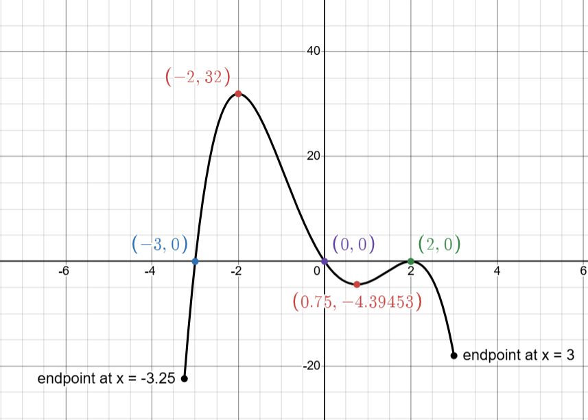
f(x) is increasing on (-3, 0), where df/dx is positive
f(x) is decreasing on (-∞, -3) U (0, ∞), where df/dx is negative
Maximums/Minimums
local maximums
x = 0, f’(x) changes from + → -
x = -3.25, left endpoint, f’(x) < 0 on (-3.25, -3)
It’s helpful to think about the sign chart. The number line would look like \ following -3.25. Because it’s to the left and approaching the right it is going up, it’s a local maximum
local minimums
x = -3, f’(x) changes from - → +
x=3, right endpoint, f’(x) < 0 on (0, 3)
It’s helpful to think about the sign chart. The line preceding 3 would look like \. Meaning that because it’s to the right and it’s going down, it would be a local minimum.
f(x) is concave up on (∞, -2) U (0.75, 2), where df/dx is increasing
f(x) is concave down on (-2, 0.75) U (2, ∞), where df/dx is decreasing
f(x) has a POIs at x = -2, 0.75, 2
Putting it all together → Derivative Analysis
We can also do this without a graph. We can now find critical information about f(x) from f’(x)
Example →
Derivative f’(x) = 4x³ - 12x²
Find critical points (f’ = 0 or DNE) →
Find the intervals where f(x) increasing/decreasing (First Derivative Test / where f’(x) > or < 0)
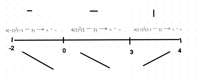
f(x) is inc → (3, 4)
f(x) is dec → (-2, 3)
Finding local extrema
local min @ x = 3, f’(x) changes from - → +
local max @ x = -2, left endpoint, f’ is - on (-2, 0)
local max @ x = 4, right endpoint, f’ is + on (3, 4)
Finding absolute extrema (candidates test)

abs min is -27 @ x = 3
abs max is 48 @ x = -2
Concavity & POI
2nd derivative → f’’(x) = 12x(x-2) → x = 0, 2

f(x) is concave up: (-2, 0) U (2, 4)
f(x) is concave down: (0, 2)
f(x) has POI @ x = 0, 2
Unit 5 - Analytical Applications of Differentiation
Velocity and Acceleration
In calculus, we can find an instantaneous rate of change.
Given the function s(t) that measures position over time, we know that the average velocity would be s(t2) - s(t1) / t2 - t1. Telling us how far it is traveled and how long the time was.
The derivatives of the position actually tell us different things
Function | What it tells us | Example of unit |
s(t) | Position | m |
s’(t) or v(t) | Velocity | m per sec |
s’’(t) or v’(t) or a’(t) | Acceleration | m per sec per sec |
Let’s try an example. In this, a heavy rock is launched straight up and it’s position function is given by s(t) = 160t - 16t²
What are the velocity and acceleration functions of time?
v(t) = 160 - 36t ft/s
a(t) = -36 ft/s²
When does the rock change direction? How high did it go?
When the sign of velocity changes, direction changes. So we need to find when v(t) = 0 and changes signs. For finding height, we simply plug the time into the position function.
160 - 36t = 0 → t = 5 seconds
So, at 5 seconds, the rocket is at 400 feet.
What is the total distance traveled between 0 < t < 7?
To find total distance, we just need to find the position at the start, end, and all the times the direction changes
First, at t = 0 seconds, s(0) = 0
Then, at t = 5 seconds (switches direction), s(5) = 400 feet
Then at t = 7 seconds, s(7) = -336 feet (going down)
Now, we add up the intervals → (0 + 400) + (400 + -336) = 464 feet
What is the speed at t = 8 seconds?
Speed is just | v(t) | so |v(8)| = 96 ft/s
Speeding Up vs Slowing Down
To find if something is speeding up or slowing down, we compare the signs of v(t) and a(t)
Speeding up → signs of v(t) and a(t) are the same
Slowing down → signs of v(t) and a(t) are opposite
Justification
(Speeding up/Slowing down) at t = time (units) because v(time) & v’(time) = a(time) (are both pos/neg / have different signs).
Velocity and Acceleration using Graphs
A velocity graph might look something like this →
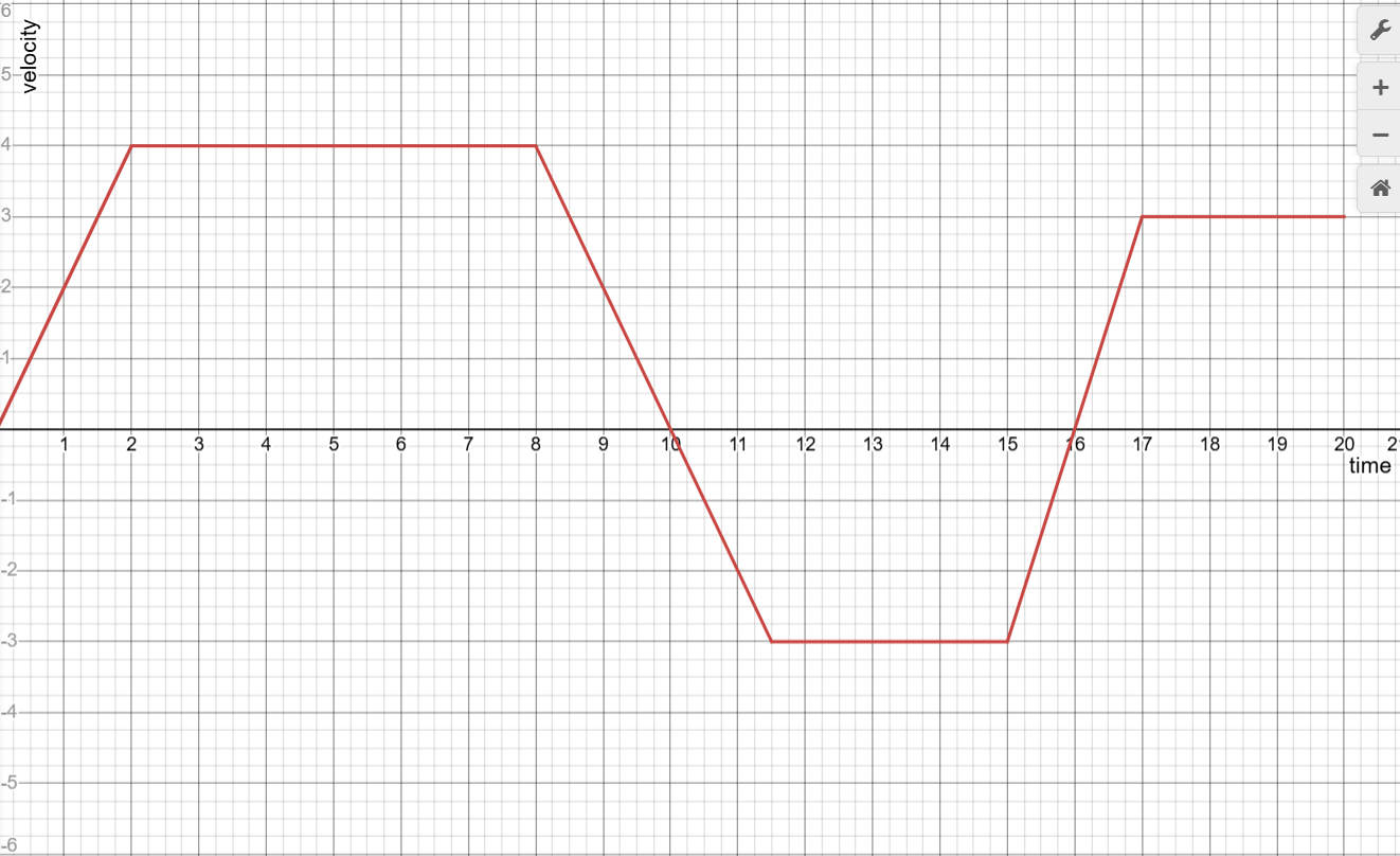
We can analyze this graph to figure out different questions. Let’s say this is the velocity of a ball floating in some random dimension from a time interval of [0, 20]
When is the ball moving forward and backwards?
It’s moving forward when v(t) > 0 so → [0, 10) U (16, 20] s
It’s moving backwards from (10, 16) s
When is the ball’s acceleration positive, negative, or zero?
For acceleration, it’s just the derivative of velocity, so we’re looking at the slope when it’s positive, negative, or zero
Positive acceleration → [0, 2) U (15, 17)
Negative acceleration → (8, 11.5)
Zero acceleration → [2, 8] U [11.5, 15] U [17, 20]
When is the ball at it’s greatest speed?
Remember, speed = |v(t)|. So → t = (2, 8)
When does the ball speed up and slow down?
Speeding up (velocity is pos & inc or neg & dec) → [0, 2) U (10, 11.5) U (16, 17)
Slowing down (velocity is pos & dec or neg & inc) → (8, 10) U (15, 16)
When does the ball change direction?
The ball changes direction when v(t) = 0 and changes signs
So t = 10, 16
What is the average acceleration between 10 < x < 13?
Average acceleration, like average velocity, isn’t using the actual acceleration function. Average acceleration uses the velocity function like so → v(t2) - v(t1) / t2 - t1
So → (0 - -3) / 10 - 13 = -1
When does the ball reach it’s highest point?
Think back to unit 4, where we found our maximums. Basically when v changes from + → -, we have a local maximum
So → t = 10
Rates of Change in Other Applied Contexts / Wording Derivatives
Here is a good explanation of a derivative in context. Make sure to give proper units, and do not phrase your description as an interval of time unless the problems calls for it.
For reference, V(t) gives rate that water fills a tank in liters per minute over t minutes modeled by the function
Find V(3) and interpret your answer.
V(3) = 9, which means at 3 minutes, the rate of which water is filling the tank is 9 liters per minute
Is the amount of water in the tank increasing or decreasing at t = 2.125 minutes?
Increasing and decreasing is just when the ROC is pos or neg. Because this function is a rate, we just need the sign of the function at t = 2.125 minutes
V(2.125) > 0, so the amount of water filling the tank is increasing.
Find V’(2.125) and interpret the value… is it increasing at an increasing rate, or increasing at a decreasing rate?
V’(t) = 2t = the rate of rate of change that water is filling the tank, measured in liters per minute²
Rate of rate of change > 0 = inc/dec @ increasing rate
Rate of rate of change < 0 = inc/dec @ decreasing rate
At t = 2.125 minutes, the rate at which water fills the tank is increasing at an increasing rate of 4.25 liters/min².
Related Rates
Related rates are basically how two rates change at the same time. You’ll often see these problems with ladders, shapes, etc. For these you’ll also need geometric formulas like for example the volume of a sphere or the surface area of a cone. Some lesser known ones may be given to you, but you should know the basic ones like area/volume of sphere and area/volume in general.
Related rates also uses implicit differentiation
There are 5 steps to solve related rates
Identify your variables, specifically your rates, and/or draw a picture. List the rates of change that you know and the rates of change you want to find given certain variables.
Write the mathematical equation that relates to your variables. Make sure to represent only the quantities that change with a variable and quantities that do not change with a constant
Differentiate both sides of your equation with respect to time
Substitute in the quantities you know at your specific time moment
Solve for the value you are seeking and interpret your solution
Examples
Shape Example → A spherical balloon is inflated with helium at a rate of 100π ft3/min. The cubed gives us a hint that this is talking about volume. How fast is the balloon’s radius increasing at the instant the radius is 5 ft?
Here’s what we know and what we need to find
Next, we use out mathematical equation for volume of a sphere and differentiate it
Now, we substitute in our values that we know to find dr/dt and solve. Our units would be ft/min because radius is a linear value
Pythagorean Example → You’re flying a kite at a height of 300 feet with the wind carrying the kite away at a rate of 25 ft/sec. How fast must you let out the string when the kite is 500 feet away from you?
Here’s a helpful picture that will assist in understanding this problem.
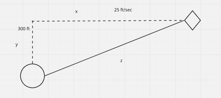
Now for our equation, Pythagoreans Theorem →
However, we’re missing our x value. At the instant when z = 500, we can use z and y (y=300) to find x →
Now we can finish solving and substituting →
Trigonometric example → A balloon, leaving the ground 60 ft from an observer, rises 10 ft/sec. How fast is the angle of elevation of the line of sight increasing when it is 12 feet in the air??
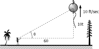
First, what we know and want to find →
Next, we need to use SOHCAHTOA. Let’s use sin because we’re given the variable y and have the rate for it.
To find the hypotenuse
Now we set up our equation and solve →
However, to find cos(theta), we use our triangle of (adj=60, opp=12, hyp=61.188). cos(theta) would be adj/hyp so that means cos(theta) = 60/61.188
L’Hopital’s Rule
Remember indeterminate limits? 0/0 and infinity/infinity? We can use derivatives to solve them. L’Hopital’s rule basically states when
Let’s see an example →
AP doesn’t really like when you write 0/0 because it techincally doesn’t exist. Instead you would write two separate limit statements of the numerator and denominator and show they are both either zero or infinity
Next, we can take the derivative of the top and bottom →
Another example →
With this example, once we simplify down the derivatives, we see that as x goes to infinity, the numerator gets bigger and bigger, meaning that we’ll have a bigger and bigger number, thus making it infinity
Unit 6 - Integration and Accumulation of Change
By taking the area of a function of velocity, let’s say at 4 seconds, the velocity is 3 ft/sec, we multiply 3 ft/sec * 4 sec = 12 feet. Finding the area under the function of v(t) gives the change in position.
Riemann Sums
We can estimate the area under a curve by taking the area of n number of rectangles from a point a to b.
There are 4 different methods of approximating the area under a curve under the interval [a, b] using a number of rectangles split into sections.
The width of each rectangle (Δx) can be found by doing this formula →
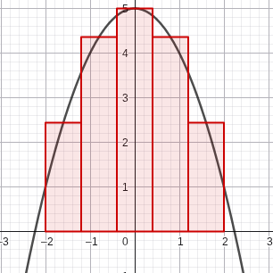
Here’s an example of each with the function f(x) = -x² + 5 with 5 rectangles:
LRAM - where we use the value of the left side to draw the rectangle.
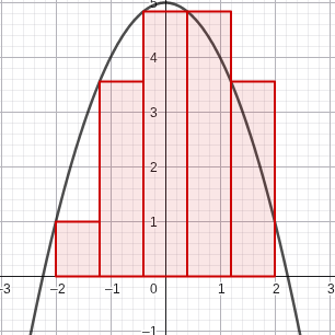
First, we have to find Δx → 2 - -2 / 5 = 4/5
Next, we start at -2 and go 4/5 until we get to 2 → (4/5)(1) + (4/5)(3.56) + (4/5)(4.84) + (4/5)(4.84) + (4/5)(3.56) = 14.24
By taking out a gcf, we get →
RRAM - where we use the value of the right side to draw the rectangle.

For this one, start at 3.56 because that is the first height → (4/5)(3.56 + 4.84 + 4.84 + 3.56 + 1) = 14.24
By taking a GCF, we get this for our RRAM →
MRAM - using the value of the midpoint between each interval to draw the rectangles.
Using MRAM, we use the midpoints in our calculation. This one’s a bit harder, but we just use the midpoint each time → (4/5)(2.44 + 4.36 + 5 + 4.36 + 2.44) = 14.88.
Trapezoidal - where we use trapezoids to measure the sum.
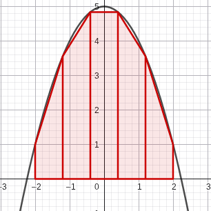
With trapezoidal sums, we use the formula for a trapezoid → , where b1 and b2 are the heights of each side of the interval, and h is your Δx. The rule can actually be simplified into this equation →
Using this, we find that the trapezoidal area would be
Usually trapezoidal is the average of LRAM and RRAM
Estimation with Table Values
More often, you can find these in tables. These may not always be in regular intervals, so you will have to do a different Δx each time. For example, let’s say this is velocity of a ball over a given time:
time (s) | 1 | 3 | 4 | 7 | 9 |
velocity (ft/s) | 5 | 9 | 12 | 13 | 4 |
Use LRAM to find the total feet traveled from t = [1, 9]:
We add up our left side values with Δx. Because our times are not at regular intervals, we have to use the length of each interval manually →
Use RRAM to to find the area from t = [1, 9]:
Do the same as before but with the right values →
Now, use TRAP to find the area from t = [1, 9]:
We can’t use our equation because of the different Δx, so we’ll have to use the area for a each individual trapezoid →
Definite Integrals
The definite integral is the area under a function f(x), from the lower limit, a, to the upper limit, b. Instead of Δx, we now have dx, where dx is an infinitely small number. The integral is basically a summation of infinitely many rectangles with a height. f(x), and infinitely small width, dx.
Properties & Rules
Here is an image of the integral →
If f(x) > 0 → is positive
If f(x) < 0 → is negative
Integrals measure exact, net area, meaning it combines the positives and negatives as they are
Here are a few rules of integrals
Transformations
Transformations in the function can be handled as such
Vertical dilation →
Vertical shift →
This is because when we raise or lower the function, we’re basically creating a rectangle under where the x-axis used to be with a width of the interval b-a and a height of the transformation c
Horizontal shift →
Horizontal dilation (you probably won’t see this) →
Indefinite Integrals / Antiderivatives
Indefinite Integrals are integrals with no bounds like this .
Integrals are actually the inverse of derivatives (which makes sense because when we multiplied the ft/sec * sec, we get the original position function of feet), called the antiderivative. Finding the antiderivative is called antidifferentiation. Meaning that…
Whenever we went down (differentiated), we denoted it by adding the prime to the little f. Now, when we climb up, we denote that as F.
Here’s an example of antidifferentiation →
The + C is there because if you differentiate the antiderivative, all constants would be 0, and we don’t know what constants are in the original function, so we put + C whenever we antidifferentiate the derivative.
We can use what we know about derivatives to “undo” the differentiation. For example, here’s how we can undo the power rule
First, add 1 to the power
Next, divide by the new power
This can also be represented as this power rule →
More Rules & Examples
When we have 1/x, the antiderivative would be ln(x), but there is a twist. When we have ln(x) as our answer, we always have to take the absolute value of x inside of ln. Here’s an example →
For exponents, if we work backwards (let’s say f(x) = 2x and f’(x) = 2xln(2)), then all we have to do is divide by the constant ln(2) to get back to 2x →
Here’s a few more examples of just regular derivatives going backwards
Using Antiderivatives for Definite Integrals (FTC)
Here is where the Fundamental Theorem of Calculus takes place. The FTC states:
With definite integrals, you don’t need to add the + C.
Let’s take this problem into account →
First, we need to find the antiderivative and evaluate it from the boundaries →
Now, we subtract F(b) from F(a) →
Here’s another problem →
Now, we can solve and follow our stepse
Limit Definition of Integral

Sometimes, you’ll see an integral defined as a reimann sum, however, it’s expressed as an infinite limit as so →
Where →
Here’s a few examples of how to convert from limit → integral and from integral → limit:
Find the limit definition of this integral →
First, we need to find our delta x →
Next, we need to find our xi →
Now, we take our function inside the integral and substitute the x’s for xi’s →
Now we need to put our limit and summation in front of the f(xi)dx →
Now, let’s turn this limit into an integral →
First, we know that in our xi, the lower bound is always first, so a=1, now we use our delta x to find our b →
Now, we substitute wherever there is an xi for an x →
Now we put our integral together →
Average Value of a Function
The average value (mean) of a function, from [a, b] is given by →
Here’s an example:
Find the average value of from [0, 3]
First, we set up our integral →
Next, we solve for our integral, keeping the 1/b-a outside to be multiplied at the end →
Now we evaluate and multiply the 1/b-a →
Fundamental Theorem of Calculus (Part II)
The fundamental theorem of calculus states that derivatives and integrals cancel each other out →
Basically, this is just rewriting the function in terms of x (or whatever variable takes the place of the d/dx). The bottom limit must always be a constant. However, there is some situations where it gets tricky →
If our upper limit is not just x, then we substitute the function for x and multiply by the derivative of the upper limit→
If our lower limit has a variable and out upper limit as a constant, we just apply our integral properties →
If both our limits are functions, then we need to basically subtract the area of the upper limit to zero (but this can be any number) from the area of the lower limit to zero →
Unit 7 - Differential Equations
Solving Integrals by U-Substitution
When solving an integral, we can undo the chain rule through something called u-substitution! If you remember the chain rule →
The steps to do u-substitution is easy!
Assign an expression to be = u (usually this is an inside function). It’s worthwhile to look for an expression who’s derivative is also in the integrand
Use the derivative of u to find a substitution for dx to du
Solve the new integral, now in terms of u
Replace u in the final answer with it’s equivalent.
Indefinite Integrals
Evaluate
First, we need our u. We’ll use 2x² since it’s the inside function →
Now, we need to take the derivative of u with respect to x →
But, we can’t have u in the integrand while we have dx, so we need to find a substitution for dx to du. Instead of thinking about du/dx as one entity, we can think of it as a fraction and multiply dx to the other side, giving us
We see that we have xdx (just switch x and cos(2x²) around because they’re multuiplied) in our problem an xdx in our du, but in order to fully substitute that, we need to just divide 4xdx by 4 and du by 4 →
We can now plug in our substitution in terms of u →
Now, we evaluate the indefinite integral in terms of u and substitute u for our original substitution (Don’t forget the + C for indefinite integrals!)→
Here’s another example →
Definite Integrals
With definite integrals, using u-sub, we just need to change the limits in terms of u.
Here’s an example →
First, we need to do our u-sub →
Next, in order to save us time, we can just plug each limit into u to get them in terms of u →
Now we solve like normal →
Here’s another example →
First, we do our u-sub with the denominator →
Now, we can actually use u to get x, so x = u - 1, and swap that in for x in our integrand →
Now, we can solve it like normal →
Differential Equations
General Solution
Differential equations are basically the opposite of implicit differentiation. There’s 4 steps
Separate your x and y and dx and dy.
Integrate both sides. Keep +C on the side with x
Rewrite in terms of y
Here’s an example:
Here’s another example
Solve the differential equation →
First, we need to seperate our dy/dx and our fraction →
Next, we integrate both sides, here we have to implement a little u-sub →
Now, we need to convert our equation back into an exponential to get rid of the log →
We can actually use our exponential properties to split our exponential. With e^C, that is just another number. Any new constants are usually denoted by A →
Now we can reduce our equation. We can also get rid of the absolute value by simply having ± on the other side, as no matter what value the right side of the equation is, the absolute value will be the same →
Now, just add one to the other side
Particular Solutions
If we are given an initial condition, or an (x, y) point that the final solution passes through, then that’s called a particular solution.
To do this, solve until we get the + C equation
Then plug in our initial condition and solve for C
Then use our new C value in the original equation
Then solve for y
The solution we find will be valid for the continuous and differentiable section of the function that involves the initial condition.
To figure out our valid domain, we will find any x-values where y is discontinuous or not differentiable. These points break our solution into pieces and the valid domain is the piece that includes our initial condition.
Examples
Find the particular solution of the differentiable equation through the point (1, 1). Indicate the domain over which the solution is valid.
First, we separate our variables →
Next, we get our equation with + C →
Now, we plug in our initial condition into x and y to get C →
Now, we plug that back into our equation with + C →
Next, we solve for y →
Now, because we have the ±, we need to plug in our x-value from the initial condition to see which one would give us the same sign as our y-value from our initial condition →
Now that we have our equation , we now have to find our domain. dy/dx is differentiable everywhere, so we’re good. Our function also exists everywhere, so our domain would be
**If it were different, then we’d have to pick the domain that includes our point
Find the particular solution of the differentiable equation through the point (0, 1/2). Indicate the domain over which the solution is valid.
First we separate and get our c equation →
Now, we solve for C →
Now, we solve for y →
Now, our domain, the inside of the log must be always > 0. Since our dy/dx is differentiable everywhere, we don’t need to do anything with that. But our domain would be → \sqrt{2x^3+e}>0\Rightarrow2x^3+e>0\Rightarrow x^3>-\frac{e}{2}\Rightarrow x>\sqrt[3]{-\frac{e}{2}}
Application of Differential Equations
In real life, separable differential equations can be used to model rate of change that is proportional to a present amount →
Solving that differential equation, we get this model for exponential change →
y is the current amount
y0 is the initial amount
k is the constant of proportionality
t is time
Here’s a few examples:
The rate of growth of the volume of a sphere is a proportional to its volume. If the volume of the sphere is initially , and expand to after 1 second, find the volume of the sphere after 3 seconds
First, we have our equation
Next, we find k →
Now, we find V at t = 3 →
Slope Fields
When we can’t algebraically seperate x and y, we can use something called a slope field, basically graphing the slope at each point by plugging the x and y values of the each coordinate into our dy/dx equation.
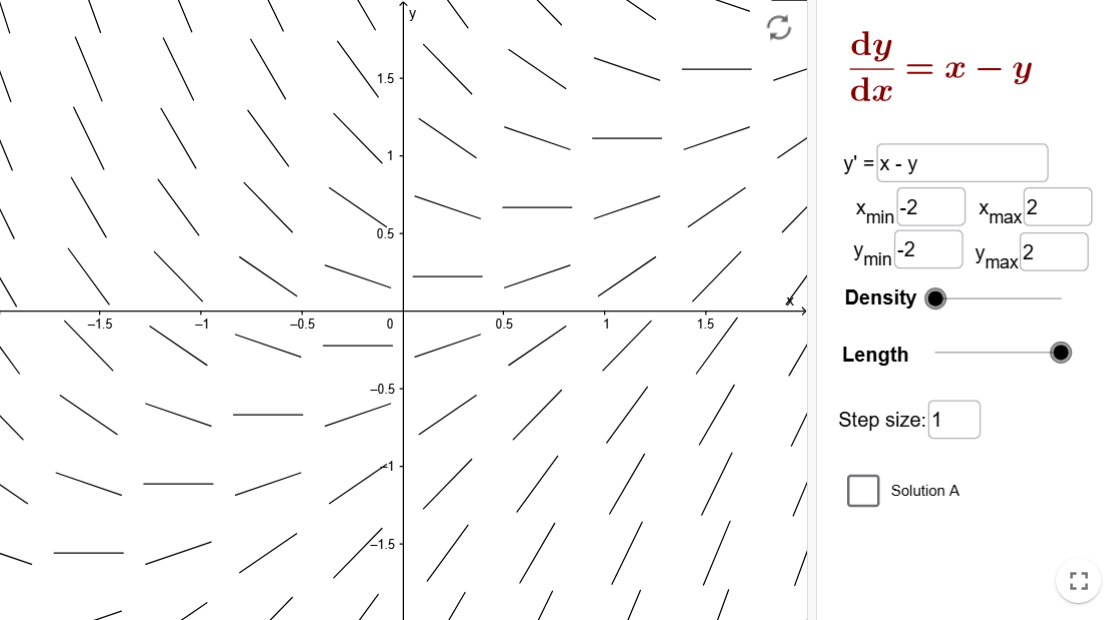
Here’s a slope field for the derivative x-y
Unit 8 - Applications of Integration
Velocity, Displacement, & Total Distance
Displacement is the net change when you integrate velocity (positive and negative)
Total Distance is the total absolute distance covered
However, we’re sometimes given the starting location, and asked to integrate over an area to find a certain new position
New Position = Old Position + Change in Position
Here’s an example:
The velocity of a particle moving along a horizontal axis for 0 < t < 5 is given by
When is the particle moving left and right?
Recall this from the old chapters, so left would be v(t) < 0 and right would be v(t) > 0
It goes left from t = [0, 1.254)
It goes right from t = (1.254, 5]
Suppose the initial position is s(0) = 14. What is the particles position at t=3
Calculate the total distance traveled by the particle in the first five seconds
Area Between Two Functions
Let’s say we want to figure out the area, sandwiched between two functions f(x) and g(x).
If we go back to how to find the area using the rudimentary definition of an integral, we need rectangles that have a length of the top function minus the bottom function. Then we’d multiply this by an infinitely thin dx width.
With function where we’re trying to find the area between f(x) and g(x), and f(x) > g(x), the area between the two curves is as so…
When working with a Top - Bottom type of area, we work in terms of x and we know to use top and bottom because the length will hit both of our rectangles. Our limits will also be in terms of x→
However, you can work from Right - Left when finding areas in terms of y. For this, we know because the length spans the two functions →
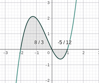
Here’s a few examples:
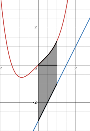
Find the area between the two functions f(x) and g(x), where f(x) = sinx + 1, g(x) = x between
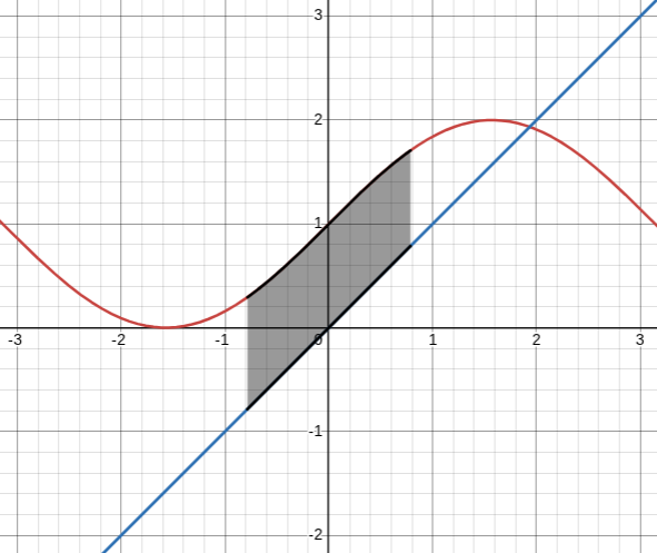
First, decide if we’re doing Top - Bottom or Right - Left. We see that going vertical would be best as the ends touch both functions and not themselves. This means we’re working in terms of x
We set up our integral →
Now, we solve →
Find the area between the functions
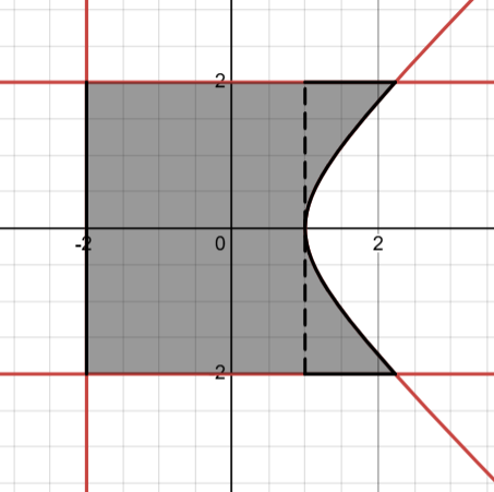
This will be horizontal, so we’re going to be working in terms of y. Since we have the limits as actual equations, and they are all y-values, we don’t have to do any converting!
It will be Right - Left so our length would be
We can set up our equation now →
Finding Volume Using Cross Sections

A cross section is a surface or shape that is or would be exposed by making a straight cut through something. We can find the volume of a shape by integrating an area function over a certain interval.
How to find Volume using Cross Sections
Sketch the base and a typical cross section based on the description
Write equation for the area of one cross section (the shape)
Find the limits of integration (If perpendicular to x → x-values, if perpendicular to y → y-values)
Integrate the area of the cross section to find the volume
Here’s a few examples:
Let R be the region bounded by x=y² and x=9. Find the volume of the solid that has R as its base whose cross sections are perpendicular to the x-axis (this means we’ll be working in terms of x).
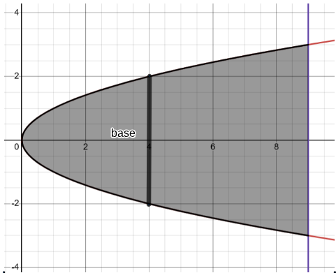
Squares with a base in the xy plane
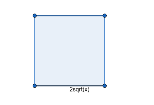
First, we need to draw the shape of the cross section. It’s base is written and would be where the thick line is on the area above
Then, we need to find the area of this cross section, as its base would be the area between the original functions. Since this is in terms of x, we have the Top - Bottom, so the length of our base would be . Now, we find our area of our square →
Now, we set up our volume integral, where we integrate the area function over the x-values of 0 to 9 because that is the bounds that were given to us→
Finally, we solve →
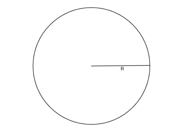
Circles with diameters in the xy plane
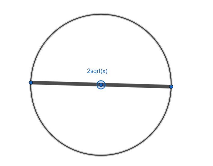
We do the same steps. First we need to find our area function →
Now we solve for our volume →
Rectangles with height of 2
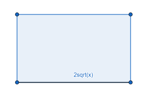
Area →
Volume →
Squares with diagonals in the xy plane
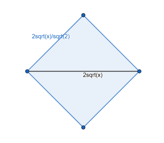
With this, we just have to divide the side lengths by sqrt(2) to find the area →
Now find the volume →
Finding Volume Using the Disk & Washer Method
Solids of Revolution are made by rotating a curve around a plane…
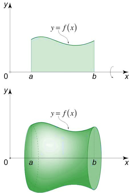
To find the volume by rotating, we can imagine taking out a circle (a disk or a washer) with the radius of f(x) and the width of dx or dy. We then add infinitely many of these disks or washers across the interval [a, b] to get our volume.
A typical cross section for a solid of revolution can be categorized as disk or washer.
A disk is when these circles are completely filled in
The area for this would be , so when we integrate our area function over [a, b] we get → , which is usually written like this →
A washer is when there is a gap in our shape and it is not filled in
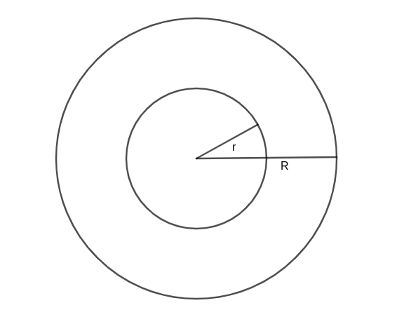
The area for this shape would be . When we integrate, we get this formula for the washer method →
When we rotate around the x-axis, we will be in terms of x
When we rotate around the y-axis, we will be in terms of y
Here’s a few examples:
x-axis
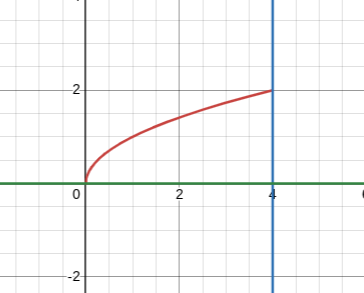
First, we see that there would be no gap between the axis of rotation, so this is a disk problem. We also know that our functions are going to need to be in terms of x since this is rotating around the x-axis
First, we find what our R would be. This would be just our Top - Bottom →
Now, our bounds are going to be x-values as well, as we know to integrate from 0 to 4. We can now write out our integral for volume →
y-axis
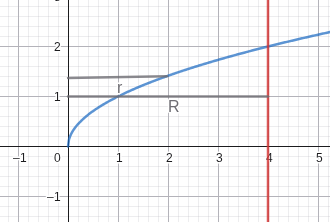
Now, because we’re rotating around the y-axis, we need our functions to be in terms of y Our boundaries are also y-values, so it goes from [0, 2] instead of [0, 4]. We also notice that there will be a space missing, so we’re going to use the washer method. First, our R goes from the farthest point to the axis of rotation, the r goes from the missing space to the axis of rotation →
Now we solve for our volume →
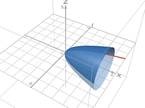
The region enclosed by y = sinx, y=cosx, x=0, is revolved around the function y = tan(x)/2
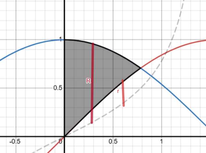
This is a washer problem. Since we’re rotating horizontally, we’ll be in terms of x. We need to find our limits, which would be x = 0 until pi/4. We need to find our big R and little r →
Now we set up our integral equation →
Now, we get our solution →
Good luck on the AP Calc AB Exam!