Corporate finance, L5
1. Options Overview
Options are financial derivatives representing contracts that grant the buyer the right, but not the obligation, to purchase (call) or sell (put) an underlying asset before or at a specific date (maturity).
1.1 Key Definitions
Call Option: Right to buy an underlying asset.
Put Option: Right to sell an underlying asset.
European Option: Can be exercised only at maturity.(discussed in this chapter)
American Option: Can be exercised any time before expiration.(discussed in the next chapter)
Exercise Price (K): The predetermined price at which the underlying asset can be bought or sold.
Premium: The cost paid by the buyer to the seller for the options contract.
2. Terminal Payoff of Options
2.1 European Call Terminal Payoff
meaning CF at maturity
Exercise Condition: If the stock price (ST) at maturity is greater than the exercise price (K)
If exercise P=100, me buyer of the call, I have the option to buy it at value 100 at maturity,
Now if it 60=price market, in this case, I don’t use my call option bc it would be cheaper directly in the market(opposite if it is 120)
Now the bold line, is the profit
Formula:
Call value at maturity: CT = MAX(ST - K, 0)
If ST > K, CT = ST - K(So if P>K, then value of call) ; otherwise, CT = 0.
Seller of Call
As a seller receives premium, but can potentially loose an infinite amount
2.2 European Put Terminal Payoff
Exercise Condition: If the stock price (ST) at maturity is less than the exercise price (K).
If K=100, want to sell at the highest value, so will not exercise on the RHS, ?
the profit is lower bc need to deduct the premium(buyer of put)
Buyer Formula:
Put value at maturity: PT = MAX(K - ST, 0)
If ST < K, PT = K - ST; otherwise, PT = 0.
3. The Put-Call Parity
3.1 Concept
The Put-Call Parity establishes a relationship between the prices of European call and put options with the same exercise price and maturity on the same stock.
→It serves as a fundamental relationship that traders use to identify mispricings in the market and take advantage of arbitrage opportunities
Strategy 1: Buy 1 share of stock and 1 put option:
If ST < K: Value = ST + (K - ST) = K
If ST > K: Value = ST + 0 = ST
→ By having portfolio of stock, when you buy a put on the specific stock then it is for protection(red line would be profit when protected, comes at a price)
Strategy 2: Buy a call option and invest PV(K) (the present value of the strike price):
If ST < K: Value = 0 + K = K
If ST > K: Value = (ST - K) + K = ST
Both strategies yield the same terminal value.
→(stock + put= Call + exercise price)
Current Value Equation
S + P = C + PV(K)
Where S = current stock price, P = current put value, C = current call value.
A call is equivalent to a purchase of stock and a put financed by borrowing the PV(K)
4. Valuing Options with the Binomial Model
4.1 Binomial Model Basics
Two state option model: Stock price can either increase (uS) or decrease (dS) over a set period.
S= non-dividend paying stock
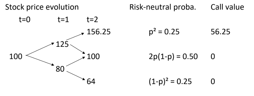
Example: Current stock price (S) = 100. If u = 1.25, then uS = 125; if d = 0.80, then dS = 80.
For a call option at K = 100:
Call values can be derived as Cu = MAX(125 - 100, 0) = 25 and Cd = MAX(80 - 100, 0) = 0.
→ By increasing the S, we increase value of call
4.2 No Arbitrage Condition
In a perfect market, the call option's value must match that of its synthetic counterpart to avoid arbitrage. (Idea is to replicate, the 25 and 0, though this synthetic call)
Call value C = δ * S - B
Calculate δ and B using pricing equations:
Solve for δ using differences in stock prices and corresponding values.
4.3 Risk-Neutral Pricing
Assumption:In a risk-neutral world, the expected return equals the risk-free rate.
risk is not numerated, bc every asset earns rf
To calculate probabilities based on potential stock price movements:
Formula: p = 0.5 for equal chances of upward and downward movements.
5. Key Parameters and Pricing Dynamics
5.1 Influencing Factors on Call Option Value
Current Stock Price (S) Call: up; Put:doxn
Exercise Price (K) Call:down; Put:up
Time to Expiry (T) call:up; Put: up
Risk-Free Interest Rate (r) call:up; Put: down
Volatility of Asset (σ) call: up; Put: up
Increased volatility typically raises option values due to heightened potential for returns without linear losses. (volatility good for options, won’t impact losses)
5.2 Black-Scholes Model
For European call options(only), represented as:
C = S N(d1) - PV(K) N(d2)
d1 and d2 calculations depend on stock price, present value of K, volatility, and time to maturity.
Black-Scholes provides a closed-form solution limiting conditions of the binomial approach, allowing for performance analytics in non-dividend stocks with constant volatility.
Moneyness of an option= will copute the gap btw S and present value K, ie. if the gap today will prbly be also pretty small in the future
6. Cumulative Normal Distribution
Utilized for calculating N(d1) and N(d2): Probabilities in standardized normal distribution contexts.
Example values can be derived using statistical functions or probability tables.