Lecture 9

HAC Standard Errors

Autocorrelation refers to the correlation of a variable with itself over time intervals (violated TS3).

• Objective: Implement statistical inference for regression coefficients under heteroskedasticity and autocorrelation.

• White's Robust Standard Error: Useful for heteroskedasticity but fails under autocorrelation. Thus, HAC SE expands by including autocorrelation when both issues present in the error terms.

• Heteroskedasticity- and Autocorrelation-Consistent (HAC) Standard Error:

  • Also known as Newey-West standard error.

  • Suitable for estimating SE(( \hat{\beta}_j )) in the presence of both heteroskedasticity and autocorrelation.

  • HAC SE is another type of robust SE.

Implementation in R

• Function: vcovHAC in the sandwich package allows for different versions of HAC standard errors.

• Example for simple regression model:
  [ yt = \alpha + \beta xt + u_t ]

• OLS estimation in R: fm = lm(y ~ x)

• HAC estimation: vcovHAC(fm)

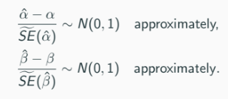
Statistical Inference Using HAC Standard Errors

• For computed HAC standard errors: [ \hat{\alpha} - \alpha \sim N(0, 1), \quad \hat{\beta} - \beta \sim N(0, 1) ]

  • Allows for standard statistical inference.

    

Asymptotic Properties of OLS Estimator

• Without normality of ( u_t ), still maintain: [ \hat{\alpha}-\alpha \sim N(0, 1) \quad \text{and} \quad \hat{\beta} - \beta \sim N(0, 1) ]

  • Valid under large sample sizes.

  • Being normally distributed for the error term (as sample size grows) and independent of X (TS6)

Conditions Under Non-Normality

• Asymptotic properties can be maintained under mild conditions.

• OLS estimators become consistent as sample size ( T ) approaches infinity.

Stochastic Regressors

• Many applications inaccurately treat regressors as non-stochastic.

• Stochastic nature means that ( E[ut|xt] = 0 ) must be satisfied for OLS estimators to remain consistent.

• The correlation between ( xt ) and ( ut ) becomes crucial.

Endogeneity

• Often arises from omitted variables or measurement error.

• Violates the exogeneity condition ( Cov(x{jt}, ut) = 0 ).

Sources of Endogeneity

1. Omitted Variable: Fails to include a relevant variable, resulting in correlated residuals.

2. Measurement Error: Improper measurement of regressors leads to correlations that disrupt consistency.

Endogeneity Bias

• Impacts the estimates: [ \hat{\beta}2 = \frac{Cov(x{2,t}, yt)}{Var(x{2,t})} ]

  • If ( Cov(x{2,t}, ut) \neq 0 ), then bias occurs. The OLS estimators become inconsistent.

Example of Endogeneity

• In empirical CAPM, substituting market portfolio returns with a specific index fund can introduce bias due to measurement error.

• If the proxy is poor, it leads to an underestimation of the actual parameters.

Instrumental Variable (IV) Estimator

• Used to address endogeneity in regression models.

• Requires a third variable (instrument) that is correlated with the regressor but not with the error term.

Confirming IV Validity and Relevance

• Validity: Requires testing that the instrument does not correlate with the error term.

• Relevance: Test whether the instrument is correlated with the regressor (i.e., usefulness of the instrument).
  [ Cov(xt, zt) \neq 0 \text{ (relevance)} \quad \text{and} \quad Cov(zt, ut) = 0 \text{ (validity)} ]

Final Notes on Inference Using IV

• If the IV method is applicable, the estimators lead to valid inferences similar to OLS under correct circumstances.

• Statistical inference can still proceed as long as the conditions of relevance and validity hold true.