IC103

Introductory Economics for Business and Finance

Lecture 6

Nur Amalina Binti Borhan

Reading (S/G/G, 10th ed.)

• Section 17.1

o except boxes 17.1, 17.2,“Looking at the Maths” in page 525.

• • Box 17.3 is optional
• Section 17.2 (including threshold concept 15),
  • “Looking at the Maths” on page 535 excluded,
  • Box 17.4 on page 537 is optional
  • Exclude “The multiplier: some qualifications” on page 537)
• Section 17.4

Section 1 National Income Determination

The circular flow of income model

3

The Circular Flow of Income INNER FLOW

Firms

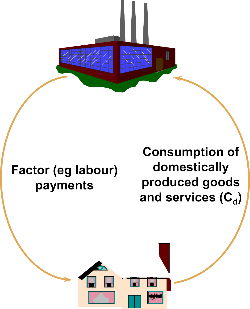
Households

The circular flow of income

Equilibrium: Withdrawals= Injections

Economy

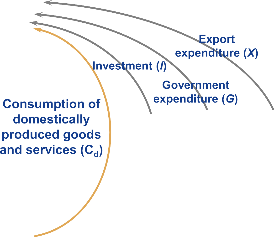
INJECTIONS

BANKS, etc

GOV.

ABROAD

Net saving (S)

Net taxes (T)

Import

expenditure (M)

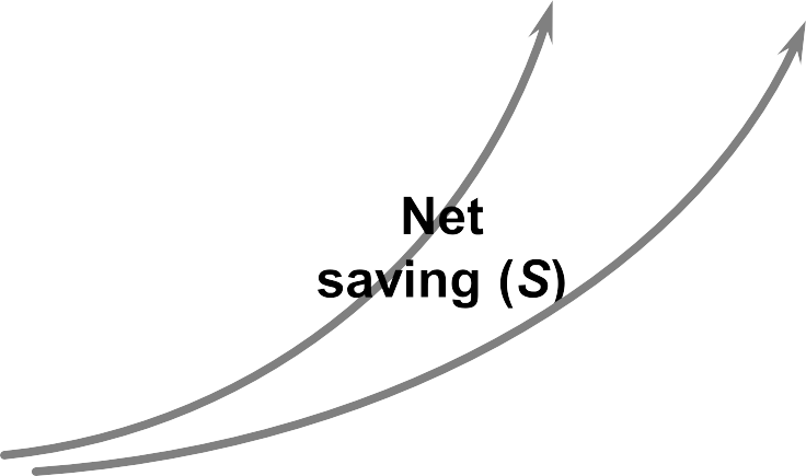
WITHDRAWALS

• Withdrawals (W)

Leakage from the circular flow, reducing the funds available for economic activity.

• • Net savings (savings minus borrowing) (S)

Saving- deposits in banks or other financial institutions

• • Net taxes (taxes minus benefits) (T)

Net Taxes = Taxes on Households - Transfer Payments

Transfer payment-social welfare program from government

• • Import expenditure (M)

Money will eventually flow out of the domestic economy to foreign producers as payments for imported goods and services.

• Injections (J)

money entering the circular flow, boosting the economic activity

• Investment (I)

Firm spending on capital goods (e.g. machinery, equipment, buildings, and infrastructure)

• Government expenditure (G)

Government spending on goods and services for public services (e.g. healthcare;

education; defence )

• Export expenditure (X)

Firms also sell goods and services abroad

Withdrawals (W)= Net saving (S) + Net taxes (T) + Import expenditure (M) Injections (J) = Investment (I) +Government purchase (G)+Export expenditure (X)

• The relationship between injections and withdrawals

Equilibrium in the circular flow: Withdrawals (W)=Injections (J)

• • If injections (J) > withdrawals(W), more spending, aggregate demand, aggregate supply national income (e.g. payment to households) and economy grows. Then S,T, M will until W=J.

Withdrawals (W)= Net saving (S) + Net taxes (T) + Import expenditure (M) Injections (J) = Investment (I) +Government purchase (G)+Export expenditure (X)

• The relationship between injections and withdrawals

Equilibrium in the circular flow: Withdrawals (W)=Injections (J)

• • If Injections (J) < withdrawals (W), less spending , aggregate demand aggregate supply, national income and economy slows, S,T, M will until W=J

Section 1 National Income Determination

The Keynesian Theory of Consumption

10

Recall: Aggregate Demand (AD)

• Total spending on goods and services made within a country Spending by consumers, businesses, the government, and foreign buyers on domestically produced goods and services (export).
• AD = C_d + I + G + X

AD = C − IM + I + G + X AD = C + I + G + X − IM =GDP

• C_domestic = C − spending on imports (IM)

Keynesian economics

Aggregate demand is the primary driver of economic activity in the short run. It determines the level of production (aggregate supply), which in turn influences national income.

• Aggregate demand, also referred to as aggregate expenditure

AD = C_d + I + G + X= C_d + Injection (I+G+X)

• National income is the total income earned by a nation’s residents in the production

of goods and services.

National income (Y) = money earned = money spent= Cd + Withdrawals (S+T+M)

• In Keynesian model, aggregate demand (AD) = national income (Y)

Injection= withdrawals

Keynesian economics

Keynes suggests:

An increase in your income (∆Y) will typically lead to an increase in your spending.

The relationship between consumption and income: Consumption (C)

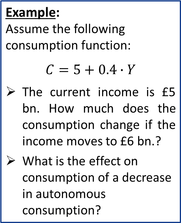
The Consumption Function

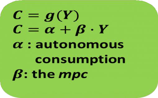
• • Consumption (C) is a function of income (C = g(Y))
  • Assume that the consumption function is linear:

C = 𝛼 + 𝛽 ∗ Y

• • 𝛼 is a constant and represents what people would consume if their disposable income equals zero (autonomous consumption).
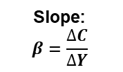
  • 𝛽 is the marginal propensity to consume (mpc): the fraction of additional current income consumed in current period. (e.g. mpc=0.5: consumption increase by £0.5 for every £1 increase in income)

mpc is equal to ΔC/ΔY (i.e., ratio of change in consumption over the change in income), positive, the slope of consumption function

Consumption Function: example

Figure: Consumption and Disposable Income

Income, Y

Consumption, C

42

50

58

66

74

82

90

98

National income

(£bn)

Consumption

(£bn)

0 10

18

34

26

10

20

30

40

50

60

70

80

90

100

110

10 + 0.8 x 60 = 58

National income

(£bn)

Consumption

(£bn)

120

Graphical Illustration

Y= C_d + W

When W=0, Y= C_d

1.The higher the income

Y of country, the more we

expect people to

100

80

Consumption (£bn)

3.The slope of consumption function

tells us how much extra income is spent on extra consumption and this is called marginal propensity to consume(MPC).

45-degree line

C

∆C = 8

∆Y = 10

60

50

₄₀ MPC = ^∆C

∆Y

=8/10= 0.8

2. Even income 0,

consumption is positive. WHY?

20

Relationship between Consumption C and domestic Consumption Cd

Y

C

C_d

C_d excludes imports

and indirect taxes.

120

100

80

Consumption (£bn)

60

40

20

Other Determinants of Consumption

• Wealth and consumers’ balance sheet
• Expected future incomes
• Availability of credit
• Consumer sentiment
• Expectations of future prices
• The age of durables
• Taxation

Section 1 National Income Determination

Withdrawals

21

Endogenous vs. Exogenous Variables

• Endogenous variables: variables depend on other variables in the model.
• Exogenous variables: variables not explained within the model but are instead taken as given.
• Withdrawals are endogenously determined

W = S + T + M, hence: mpw = mps + mpt + mpm

Y = Cd + W, hence: mpcd + mpw = 1

The W and Cd Functions

C_d, W

2. When domestic consumption equal to income, withdrawal must be 0, so the slope of the withdrawal functions will be different from the consumption

function.

C_d + W (=Y)

100 Cd

3. Note that given 70

that there

is positive

consumption at 0 W

wealth, there must

been negative withdrawals at 0 wealth.

30

O 100 Y

Section 1 National Income Determination

Injections

26

Injections

• Injections (exogenously determined)
  • Unlike withdrawals, Constant in relation to income (not determined by income)
• Investment (I)
  • Increased consumer demand
  • Expectations
  • Credit and interest rates
• Government expenditure (G)
• Determinants: Government objectives (short- and long- run)
• Exports (X)
• Determinants: foreign incomes, exchange
  • Cost and efficiency of capital equipment

rates, relative product quality, other

Section 1 National Income Determination

Equilibirum

28

Injections and Withdrawals Functions

C_d, W, J

Equilibrium national income:

W=J

W

J

O Y

C_d, W, J

O

If injections exceed withdrawals,

national income will rise.

J>W, economy will produce more to satisfy

additional expenditure, incomes will rise, more savings, taxes, imports hence W rise (do not forget: W=g(Y))

W

a

J>W

J

b

Y₁

Y

C_d, W, J

O

If withdrawals exceed injections,

national income will fall.

J<W, economy will produce less as there is

deficient expenditure, incomes will fall, less

savings, taxes, imports hence W fall

W

c

d

J

J<W

Y₂

Y

C_d, W, J

O

Equilibrium national income

is where W = J.

W

x

J

Ye

Y

C_d, W, J

If aggregate expenditure exceeds national income, national income will rise.

Y = Cd + W

E = C_d + J = AD

C_d

J also

above W e

W

f

J

O Y1 Y

If national income exceeds

aggregate expenditure, national income will fall.

Y = C_d + W

g

h

E = C_d + J

C_d

W

J

Y₂

Y

J also below W

C_d, W, J

O

Equilibrium national income is

where Y = E (and W = J).

Y = C_d + W

E = C_d + J

C_d

z

W

x

J

Ye

Y

O

Equilibrium National Income

• Equilibrium national income
  • Withdrawals equal injections
• Income equals expenditure

Section 2 National Income Determination

The Multiplier

37

Determination of National Income

An increase in the income (∆Y) will typically lead to an increase in consumption (ΔC).

An increase in injection(∆J ) will typically lead to an increase in the income (∆Y).

∆J ∆Y ΔC

Consumption

• The multiplier

The multiplier

function

• • The ratio of the change in income relative to the change in injections (i.e.

∆Y/∆J)

Cumulative causation: an initial event can lead to successive changes in other institutions.

The Multiplier: A Shift in Injections (I)

W, J

W

a

J₁

Ye

Y

O

W, J

The Multiplier: A Shift in Injections (II)

If gov increase spending, by investing in infrastructure project, this create additional revenue for business. These businesses need to use additional labor. So, therefore, provide additional income to the household. Then, household spends more which leads to additional revenue to the firm. So J increase from J1 to J2.

How much extra income does this processWcreate?

b

J₂

a

J

1

O Ye Ye Y

W, J

Multiplier = ΔY / ΔJ

= ΔY / ΔW

= c – a / b – c

• • • This diagram shows that the

change in J = change in W.

• • • The withdrawal function is change in W divide by change in Y.
    • The multiplier is the inverse of this.

J₂

ΔJ a

J₁

O Ye

W

b

J₂

ΔW

J

c 1

ΔY Ye Y

W, J

Multiplier = ΔY / ΔJ

= ΔY / ΔW

= c – a / b – c

= 1/mpw

b

ΔJ

a

ΔW

c

W

J₂

J

1

Ye

ΔY

Ye

Y

J₂

1

J

O

Multiplier Formulas

• The multiplier is defined as follows:

k = 1/mpw

• Since: mpw + mpcd = 1 it follows that

k = 1/(1 − mpcd)

• From the above:
• The greater the mpw, the lower the multiplier
• The greater the mpcd, the greater the multiplier

2 80 40

40

4 20 10

10

6 5 2.5

2.5

  

5 10 5 5

3 40 20 20

Round

ΔJ (£m)

ΔY (£m)

ΔCd (£m)

ΔW (£m)

1

160

160

80

80

4 20 10

10

6 5 2.5

2.5

  

5 10 5 5

3 40 20 20

Example: The Multiplier

4 20 10

10

6 5 2.5

2.5

  

5 10 5 5

Example: The Multiplier

6 5 2.5

2.5

  

5 10 5 5

6 5 2.5

2.5

  

1

2

160

160

80

80

40

80

40

Round

ΔJ (£m)

ΔY (£m)

ΔCd (£m)

ΔW (£m)

3

4

5

40

20

10

20

10

5

20

10

5

1   320 160

160

  

1

2

160

160

80

80

40

80

40

3

4

5

40

20

10

20

10

5

20

10

5

Round

ΔJ (£m)

ΔY (£m)

ΔCd (£m)

ΔW (£m)

6

5

2.5

2.5

1

2

160

160

80

80

40

80

40

Round

ΔJ (£m)

ΔY (£m)

ΔCd (£m)

ΔW (£m)

3

4

40

20

20

10

20

10

  

5

6

10

5

5

2.5

5

2.5

1  

320

160

160

W, J

Withdrawals Multiplier

O

A shift in withdrawals

Multiplier = ΔY / ΔW

= c – a / a – b

a

c

W₁

W₂

J

ΔW

b

Ye1

ΔY

Ye2

Y

Section 3 National Income Determination

The Accelerator

52

Keynesian Analysis of the Business Cycle

• The accelerator
  • Instability of investment
  • Changes in the national income and induced investment
  • The accelerator coefficient (): It = 𝛼 ∆Y
  •  depends on marginal capital/ output ratio
    • Extra investment (I) or change in capital (∆K) to achieve the production of extra output or income ∆Y

Fluctuation in UK Real GDP and Investment

30

GDP

Investment

20

10

Annual % change

0

-10

-20

1960 1965 1970 1975 1980 1985 1990 1995 2000 2005 2010

Source: Based on data in United Kingdom Economic Accounts (National Statistics)

The Accelerator Effect (I)

Year

(extra machines)

The Accelerator Effect (II)

Year

investment (I_r)

The Accelerator Effect (III)

Year

Period t J   Y  (Multiplier)

Period t + 1 Y   I  (Accelerator)

I   Y  (Multiplier)

Period t + 2 If  Y_{t +1} >  Y_t then I 

If  Y_{t +1} =  Y_t then I stays the same (Accelerator) If  Y_{t +1} <  Y_t then I 

This in turn will have a multiplied

upward effect, no effect, or a (Multiplier) multiplied downward effect

respectively on national income.

Period t + 3 This will then lead to a further

accelerator effect and so on . . .

Period t

J   Y 

(Multiplier)

Period t + 1 Y   I 

I   Y 

Period t + 2 If  Y_{t +1} >  Y_t then I 

If  Y_{t +1} =  Y_t then I stays the same (Accelerator) If  Y_{t +1} <  Y_t then I 

This in turn will have a multiplied upward effect, no effect, or a

multiplied downward effect (Multiplier)

respectively on national income.

Period t + 3 This will then lead to a further

accelerator effect and so on . . .

(Accelerator) (Multiplier)

Period t + 1 Y   I 

I   Y 

(Accelerator) (Multiplier)

Period t + 2

If  Y_{t +1} >  Y_t then I 

If  Y_{t +1} =  Y_t then I stays the same If  Y_{t +1} <  Y_t then I 

This in turn will have a multiplied upward effect, no effect, or a multiplied downward effect respectively on national income.

Period t + 3 This will then lead to a further

accelerator effect and so on . . .

(Accelerator)

(Multiplier)

Period t + 1 Y   I 

I   Y 

Period t + 2

If  Y_{t +1} >  Y_t then I 

If  Y_{t +1} =  Y_t then I stays the same

If  Y_{t +1} <  Y_t then I 

(Accelerator)

This in turn will have a multiplied

upward effect, no effect, or a multiplied downward effect respectively on national income.

(Multiplier)

(Accelerator) (Multiplier)

Period t + 3 This will then lead to a further

accelerator effect and so on . . .

Reference

• Sloman, J., Wride, A. and Garratt,D (2018) “Economics” (10th edition)
• Gregory, Mankiw, N. (2017) “Economics” Cengage Textbooks
• Symeonidis, Lazaros (2022) IC103 Introductory Economics for Business and Finance materials