Ch4 Regression Models

Chapter 4: Regression Models

• Course: ISOM 201 Data & Decision Analysis

• Instructor: Dr. Yuanxiang John Li

• Affiliation: Sawyer Business School, Suffolk University, Boston

4.1 Chapter Outline

• 4.1 Scatter Diagrams: Visual tool to show relationships between variables

• 4.2 Simple Linear Regression: Involves one dependent and one independent variable

• 4.3 Measuring the Fit of the Regression Model: Techniques to evaluate model performance

• 4.4 Assumptions of the Regression Model: Necessary conditions for valid statistical tests

• 4.5 Testing the Model for Significance: Assessing the relationship between variables

• 4.6 Using Computer Software for Regression: Use of software tools for analyses

• 4.7 Multiple Regression Analysis: Models incorporating multiple independent variables

• 4.8 Binary or Dummy Variables: Treatment of qualitative data in regression

• 4.9 Model Building: Strategies for constructing effective models

• 4.10 Nonlinear Regression: Models addressing non-linear relationships

• 4.11 Cautions and Pitfalls in Regression Analysis: Important considerations and common mistakes

4.2 Introduction to Regression Analysis (1 of 2)

• Purpose of Regression Analysis:

  • An invaluable tool for managers.

  • Used to understand relationships between variables.

  • Utilize in predicting variable values based on others.

• Types of Regression Models:

  • Simple Linear Regression: Contains only two variables (one dependent and one independent).

  • Multiple Regression Models: Involves more than one independent variable.

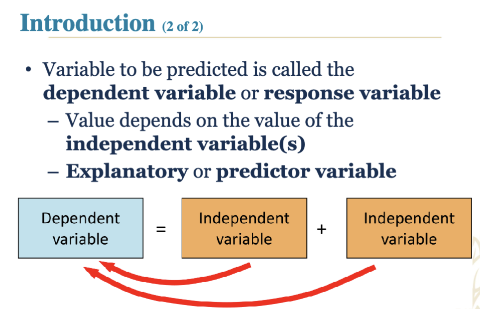
4.3 Introduction to Regression Analysis (2 of 2)

• Dependent Variable:

  • Also known as the response variable.

  • Its value is influenced by the independent variable(s).

• Independent Variable(s):

Known as predictor or explanatory variables, they are used to predict the dependent variable.

• Explanatory or Predictor variable

4.4 Scatter Diagram

• Definition: A graphical representation to investigate relationships between variables.

  • Axes:

  • Independent variable plotted on the X-axis.

  • Dependent variable plotted on the Y-axis.

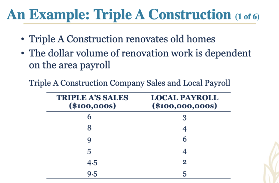
4.5 Example: Triple A Construction (1 of 6)

• Case Context:

  • Triple A Construction specializes in home renovation.

  • The renovation dollar volume depends on the area payroll.

    

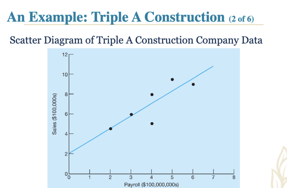
4.6 Example: Triple A Construction (2 of 6)

• Data Representation: Scatter diagram is created from company sales versus local payroll data.

  

4.7 Simple Linear Regression (1 of 2)

• Model Structure:

  • Simple linear regression has one dependent and one independent variable:

    • Y = β0 + β1X + e

      • Y: dependent variable (response)

      • X: independent variable (predictor)

      • β0: intercept (Y value when X = 0)

      • β1: slope of the regression line

      • e: random error.

4.8 Simple Linear Regression (2 of 2)

• Estimation:

  • True values of slope (β1) and intercept (β0) are unknown but estimable from sample data:

    • Ŷ = b0 + b1X

      • Ŷ: predicted value of Y

      • b0: estimate of β0 from sample

      • b1: estimate of β1 from sample.

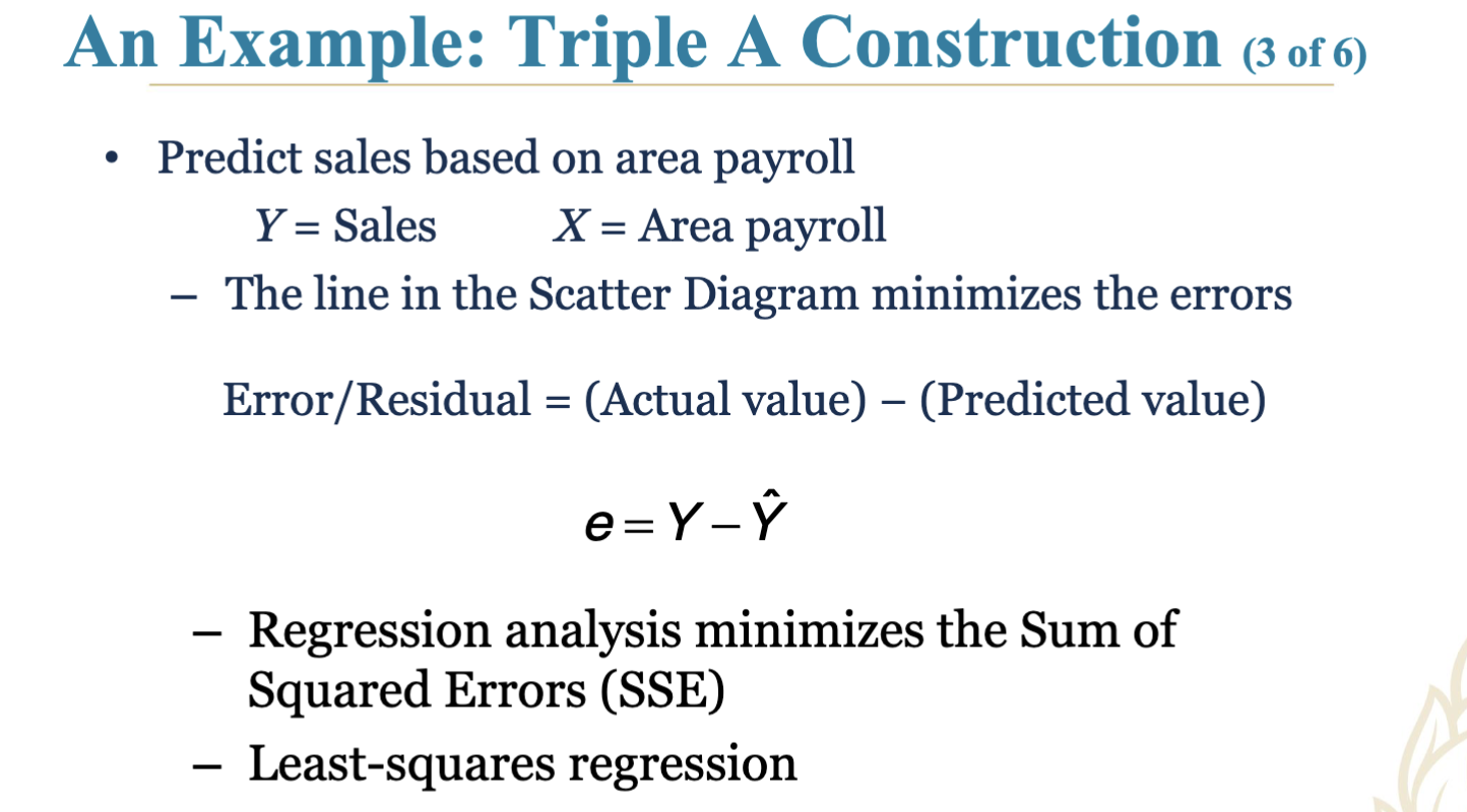
4.9 Example: Triple A Construction (3 of 6)

• Prediction Setup:

  • Predict sales from area payroll.

  • Errors/Residual: Actual value minus Predicted value.

  • Regression analysis utilizes the least-squares approach to minimize Sum of Squared Errors (SSE).

    

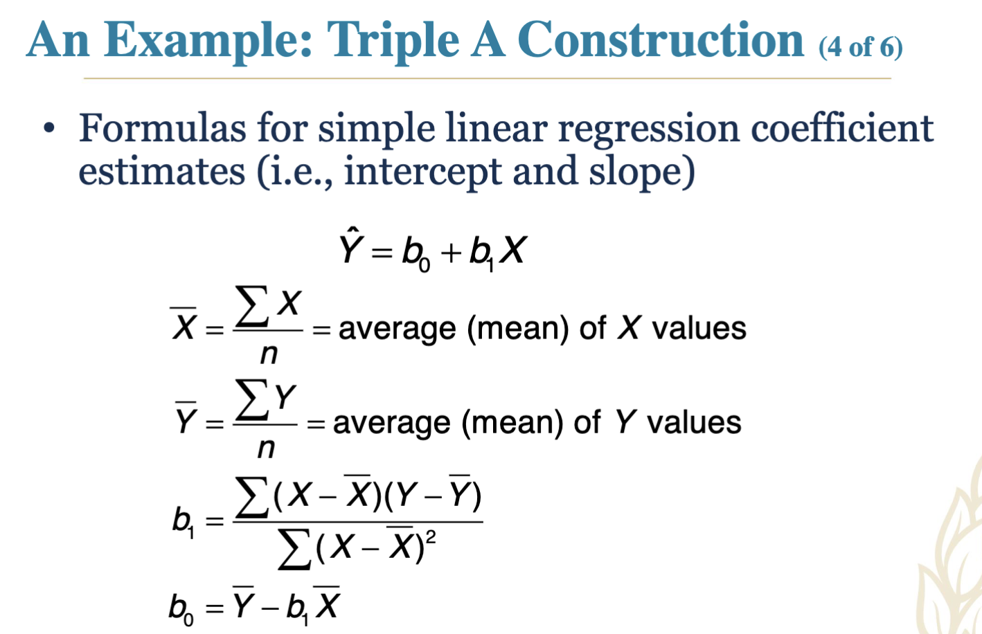
4.10 Example: Triple A Construction (4 of 6)

• Formula Assumptions: Coefficient estimates for simple linear regression are calculated using the averages of values:

  • Sample means for Y (Sales) and X (Payroll) are used to calculate estimates.

    

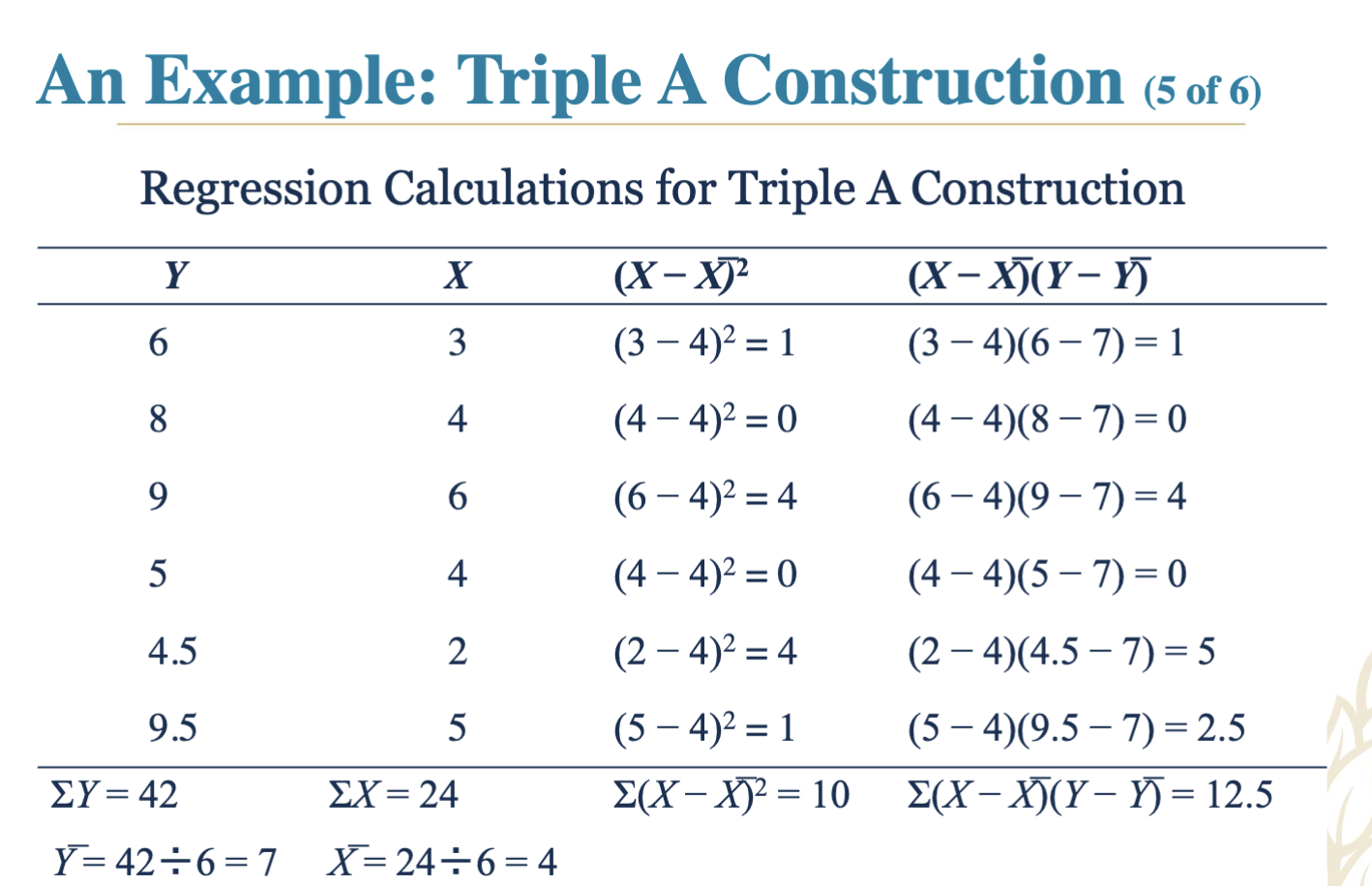
4.11 Example: Triple A Construction (5 of 6)

• Regression Calculation Insights:

  • Computation for regression coefficients and analysis of the variance in Y scores.

    

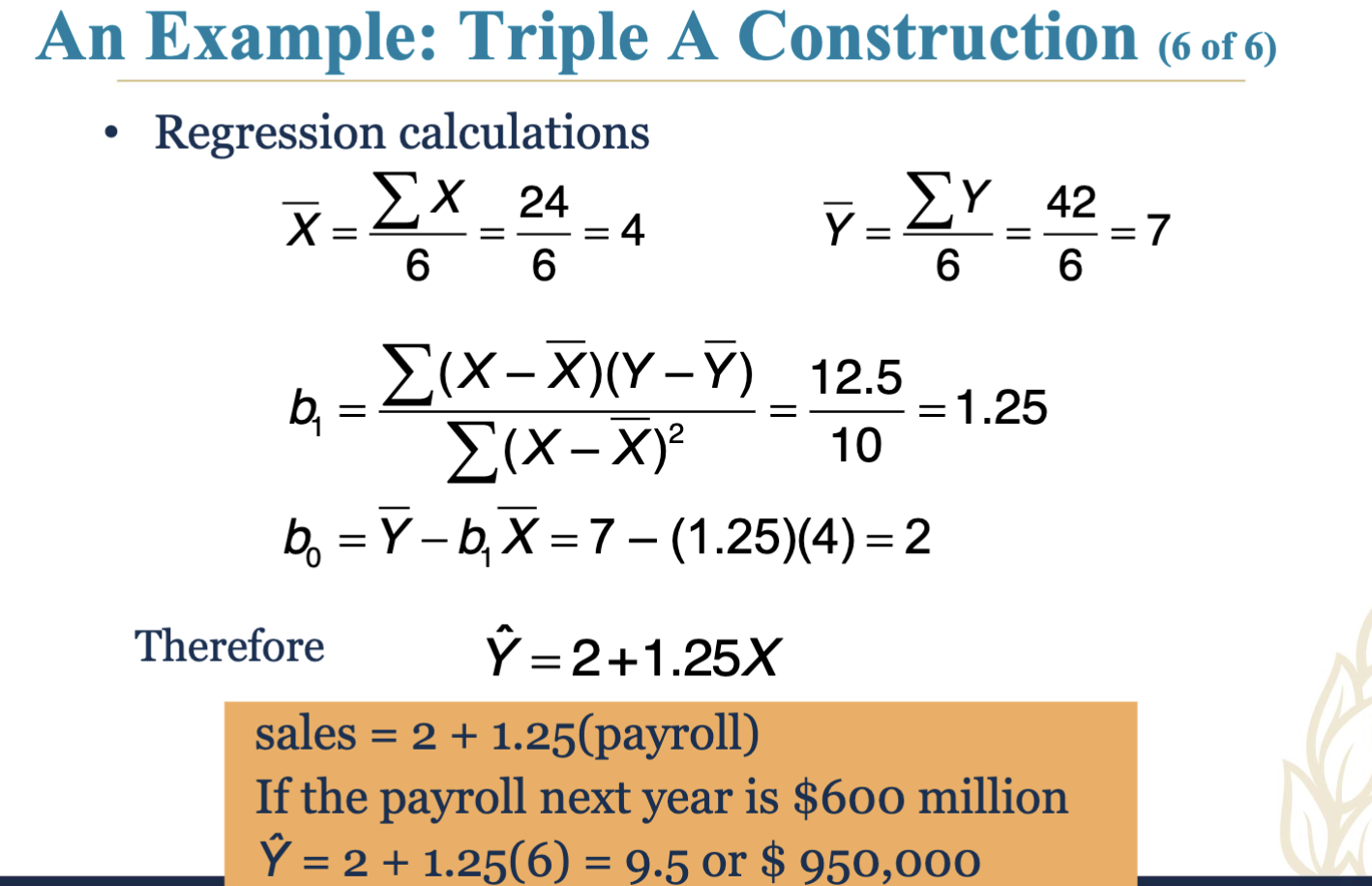
4.12 Example: Triple A Construction (6 of 6)

• Final Model Output:

  • Resulting regression model: Sales = 2 + 1.25(Payroll).

    

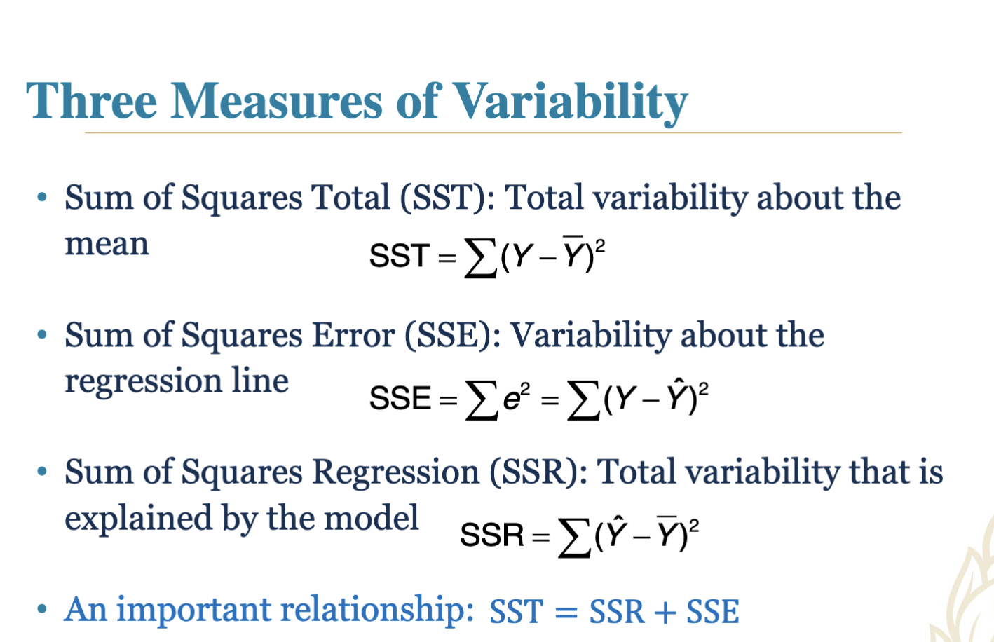
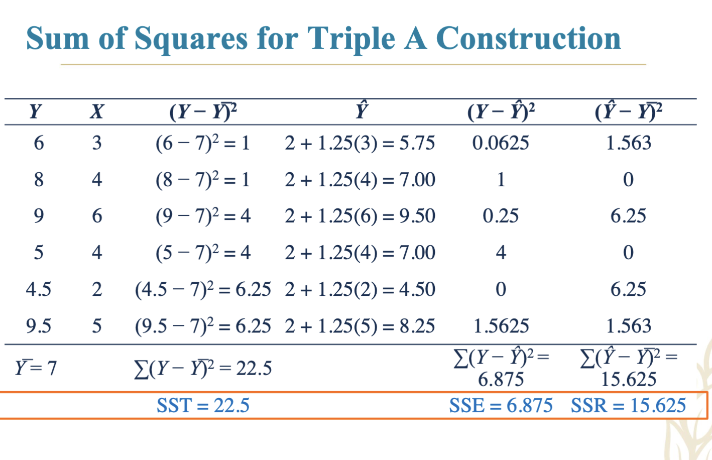
4.13 Three Measures of Variability

• Sum of Squares:

  • Total Sum of Squares (SST): Total variability around the mean.

  • Sum of Squares Error (SSE): Variability around the regression line.

  • Sum of Squares Regression (SSR): Variability explained by the model.

  • Relationship: SST = SSR + SSE

    

4.14 Example: Sum of Squares for Triple A Construction

• Detailed statistical breakdown of Y, X, and their variances related to regression.

  

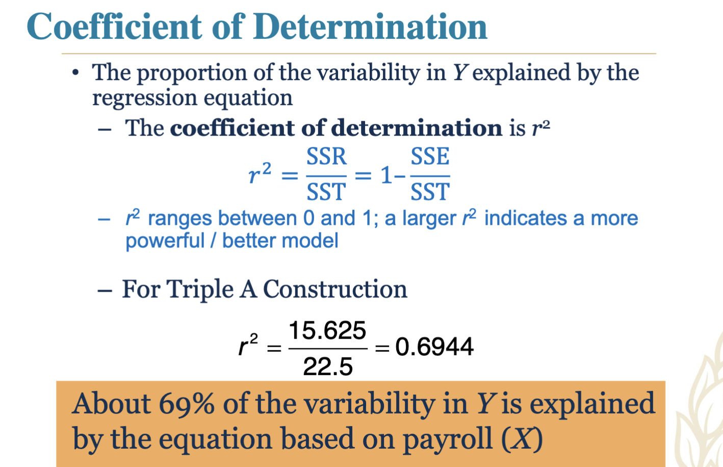
4.15 Coefficient of Determination

• Definition: Proportion of variability in Y explained by the regression model.

  • Range: 0 to 1; higher values indicate a better-fitting model.

  • Example for Triple A Construction: r² is approximately 0.6944, indicating that about 69% of the variability in sales is explained by payroll.

    

4.16 Correlation Coefficient

• Definition: Measures strength of linear relationships, ranging between +1 and -1.

  • Example calculation for Triple A Construction yields r = 0.8333.

4.17 Assumptions of the Regression Model

• Key Assumptions:

  1. Errors are independent.

  2. Errors are normally distributed.

  3. Errors have a mean of zero.

  4. Errors have constant variance.

  • Residual plots can highlight violations of these assumptions.

4.18 Additional Topics Covered

• Error Residual analysis through various plots.

• Variance estimation methods using Mean Squared Error (MSE).

4.19 Hypothesis Testing Framework

• General procedure for hypothesis testing around regression models, considering null and alternative hypotheses as well as F-statistics.

4.20 Multiple Regression Analysis (1 of 2)

• Expansion of simple linear regression to include multiple independent variables with a defined relationship.

4.21 Multiple Regression Analysis (2 of 2)

• Estimation process of parameters using data samples in a multiple regression framework.

4.22 An Example: Jenny Wilson Realty (1 of 6)

• Establish a model to suggest pricing based on house size and age metrics.

4.23 Data Presentation: Jenny Wilson Real Estate

• Information on properties sold, including selling price, square footage, condition, etc.

4.24 Evaluating the Multiple Regression Model (1 of 2)

• Similarities and differences in evaluating significance in multiple regression compared to simple models using p-values and hypothesis testing.

4.25 Final Thoughts on Multiple Regression Analysis (2 of 2)

• Consideration of significance for each independent variable in predicting outcomes for real estate pricing.

4.26 Understanding Binary or Dummy Variables

• Definition: Created for qualitative data, allowing for inclusion of categorical variables (e.g., condition types) within the regression framework.

4.27 Example: Utilizing Dummy Variables in Jenny Wilson Realty

• Implementation of dummy variables to enhance model predictions regarding house condition.

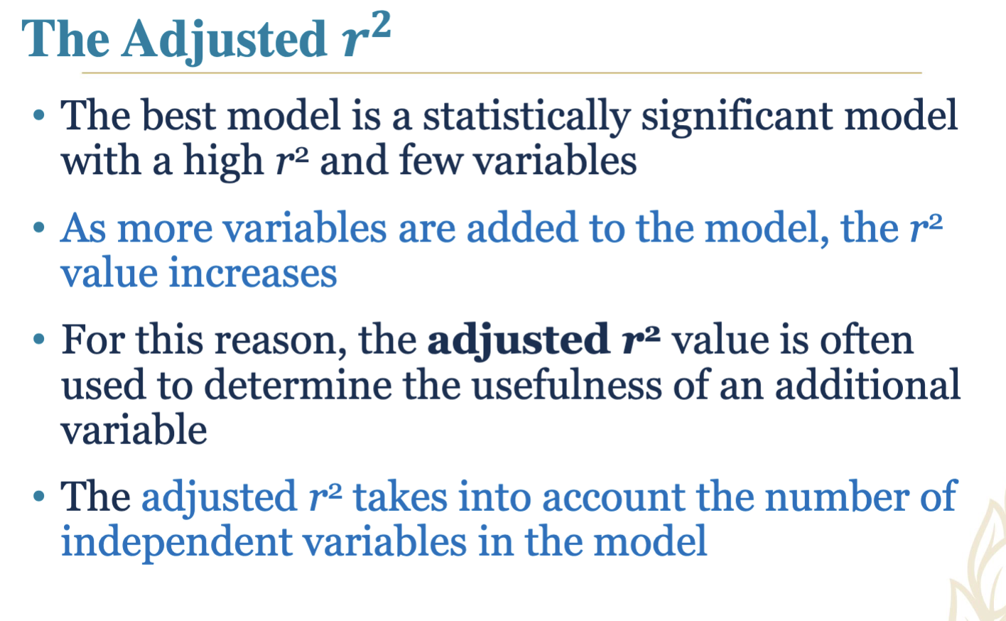
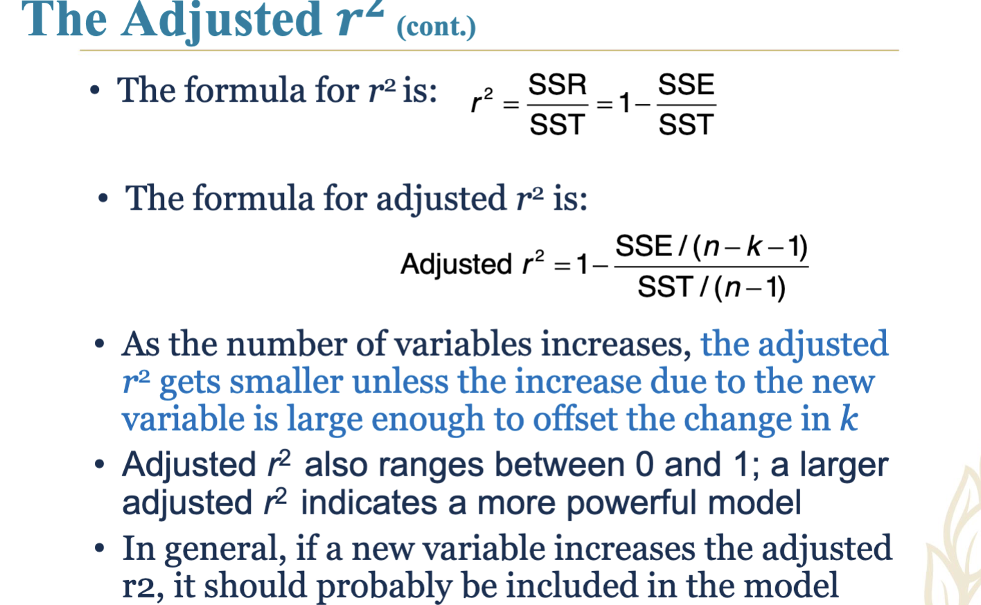
4.28 Adjusted r² as a Model Evaluation Metric

• Importance of adjusted r² over regular r² for assessing model accuracy, particularly with added variables.

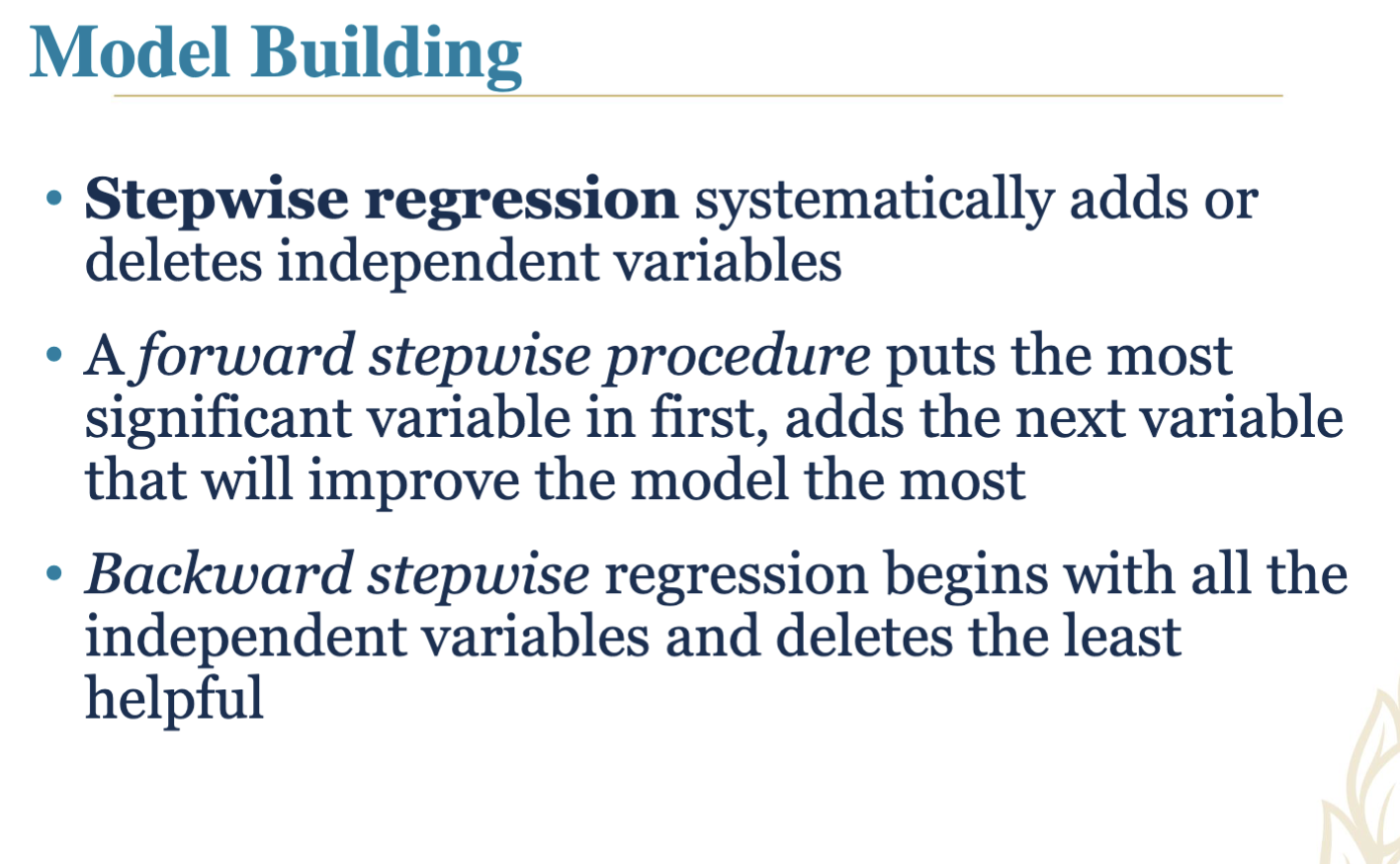
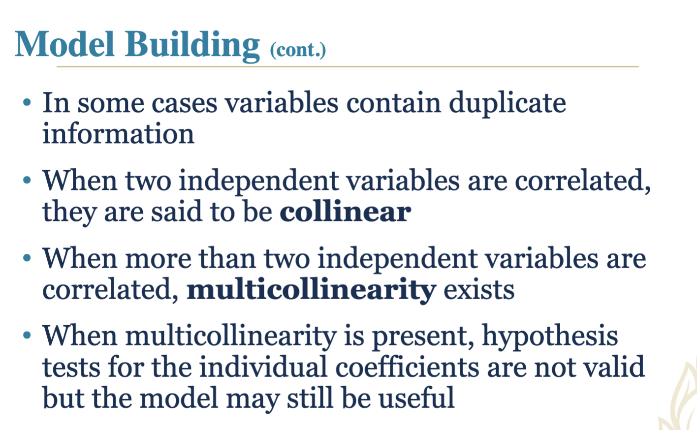
4.29 Model Building Techniques

• Stepwise regression methodologies including forward and backward steps to enhance predictive modeling.

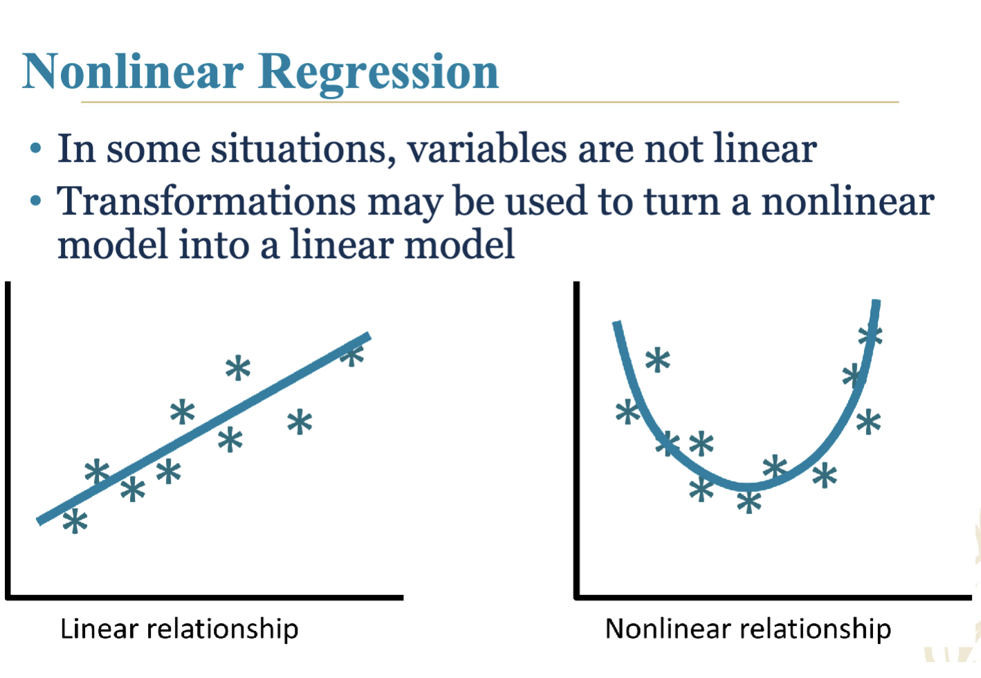
4.30 Nonlinear Regression Models

• Introduction and methods for transforming non-linear relationships into linear models for ease of analysis.

4.31 Case Study: Colonel Motors

• Analyzing the impact of weight on fuel efficiency (MPG) using regression techniques.

4.32 Considerations and Limitations

• Cautions regarding invalid statistical tests, correlation vs. causation, various regression pitfalls, and modeling beyond known data ranges.