unit 2 to unit 7

UNIT 2 — Social Interactions & Economic Outcomes

1. Self-Interest and Social Outcomes

Self-interest does not always lead to socially optimal outcomes.

• Good outcomes → Invisible Hand

• Bad outcomes → Prisoner’s Dilemma, Tragedy of the Commons

Why bad outcomes occur:

• Individuals care only about own payoffs

• No mechanism to make players internalise effects on others

• No coordination before decisions

• One-shot interactions

2. Social Preferences

Social preferences: individuals care about their own payoff AND others’ payoffs.

Types:

• Altruism – helping others at a cost to yourself

  • e.g. paying taxes honestly, environmental behaviour

• Inequality aversion – dislike unequal outcomes

• Reciprocity – respond kindly to kindness, punish unkindness

• Social norms – shared rules of acceptable behaviour

How economists study preferences:

• Surveys (subjective)

• Observational data (hard to control)

• Lab experiments (controlled, replicable)

• Field experiments (more realistic)

3. Repeated Games & Cooperation

In repeated interactions, better outcomes can arise because:

• Future consequences matter

• Social norms develop

• Reciprocity and punishment deter selfish behaviour

Peer Punishment

• Players can pay to punish free-riders

• Punishment is altruistic (costly to punisher)

• Increases cooperation in public goods games

4. Nash Equilibrium (NE)

Nash equilibrium: a set of strategies where no player can benefit by changing their strategy alone.

Key points:

• A player does not need a dominant strategy

• NE may be inefficient

5. Multiple Nash Equilibria & Conflict

When there are multiple NEs:

• Which one occurs?

• Is there a conflict of interest?

Climate Change Game

• Two NEs: one country restricts emissions, the other free-rides

• Everyone wants to avoid catastrophe

• Each wants the other to move first

• Explains difficulty of international agreements

Policy goal: change the game so (Restrict, Restrict) becomes a NE

UNIT 3 — Public Policy, Fairness & Efficiency

1. Evaluating Economic Outcomes

Two key criteria:

• Efficiency

• Fairness

Pareto Efficiency

An allocation is Pareto efficient if:

⚠ Pareto efficiency says nothing about fairness
→ Extremely unequal outcomes can still be Pareto efficient.

2. Ultimatum & Dictator Games

Ultimatum Game

• Proposer offers a split

• Responder can accept or reject

• Rejection → both get nothing

Insight:

• Pure self-interest predicts acceptance of any offer

• In reality, unfair offers are often rejected → social preferences

Dictator Game

• Responder cannot reject

• Efficient but often unfair

➡ Shows trade-off between efficiency and fairness

3. Fairness: Substantive vs Procedural

Substantive Fairness

• Concerned with outcomes

• How unequal are the final allocations?

Procedural Fairness

• Concerned with process

• Were rules impartial, transparent, and voluntary?

Example: “I cut, you choose”

• Equal outcome

• Fair procedure
  → Generally seen as fair

4. Rawls’ Veil of Ignorance

Evaluate policies as if you do not know your position in society:

• Rich or poor

• Healthy or ill

• Male or female

Encourages impartial judgement of institutions and policies.

5. Public Policy Tools

Policies influence behaviour by changing:

• Directives (rules)

• Incentives (taxes, subsidies)

• Information

Example: Overgrazing Tax

• Forces individuals to internalise social costs

• Fair (applies equally)

• Efficient (less skilled farmers exit)

6. Unintended Consequences

Policies can:

• Crowd out social norms

• Change preferences

Examples:

• Fines for late pickup at daycare increased lateness

• Seatbelts → riskier driving

• Legal drinking age → marijuana use

Good policy design requires:

• Intended outcome is a Nash equilibrium

• Preferences are not undermined

UNIT 4 — Work, Wellbeing & Scarcity

1. Scarcity & Choice

Individuals want:

• More consumption

• More free time

But consumption requires work → trade-off.

2. Production Function

Shows how inputs → outputs (holding other factors constant).

Key concepts:

• Marginal product: extra output from extra input

• Diminishing marginal product: productivity falls as input rises

3. Feasible Frontier & MRT

• Feasible frontier: all possible combinations

• MRT (Marginal Rate of Transformation):

  • Slope of feasible frontier

  • Measures opportunity cost

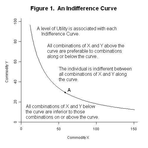
4. Indifference Curves & MRS

• Indifference curves show equal utility

• MRS (Marginal Rate of Substitution):

  • Slope of indifference curve

  • Willingness to trade one good for another

Properties:

• Downward sloping

• Higher curves = higher utility

• Do not cross

5. Optimal Choice

Utility maximisation occurs where:

Graphically:

• Tangency between indifference curve and feasible frontier

UNIT 5 — Institutions, Power & Inequality

1. Institutions

Institutions = written and unwritten rules shaping interaction and distribution.

They determine:

• Incentives

• Power

• Allocation of surplus (rents)

2. Power

Power = ability to influence outcomes against others’ interests.

Forms:

• Take-it-or-leave-it offers

• Threat of imposing costs

Property rights are a key source of power.

3. Angela & Bruno Model

Shows how allocations differ under:

• Force

• Property rights

• Rule of law

Key insight:

• Voluntary agreements shrink total surplus

• But improve welfare for the weaker party

UNIT 6 — Firms: Workers, Managers & Owners

1. Firms vs Markets

Markets:

• Decentralised

• Voluntary exchange

Firms:

• Centralised authority

• Orders replace prices

2. Incomplete Contracts

Labour contracts are incomplete because:

• Effort is hard to measure

• Future contingencies unknown

3. Employment Rent

Employment rent:

Employment rent =
Wage − disutility of effort − reservation wage

Higher rent:

• More effort

• More employer power

Unemployment benefits reduce employment rent → lower effort.

UNIT 7 — Firms & Markets for Goods

1. Economies of Scale

Large firms may be more profitable due to:

• Specialisation

• Bulk buying

• Network effects

But can suffer diseconomies of scale (bureaucracy).

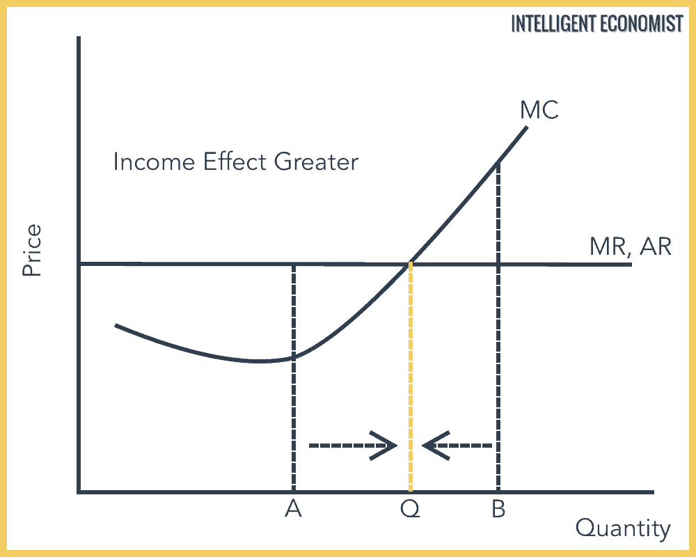
2. Profit Maximisation

Two equivalent conditions:

• MRS = MRT

• MR = MC

Demand curve = feasible frontier
Isoprofit curves = indifference curves

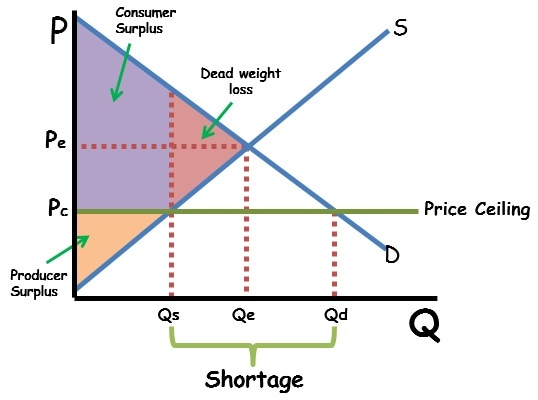
3. Surplus & Deadweight Loss

• Consumer surplus = WTP − price

• Producer surplus = price − MC

• Total surplus = CS + PS

Deadweight loss occurs when:

• Price ≠ Marginal Cost

• Gains from trade are not fully realised

4. Price Elasticity of Demand

Elasticity affects:

• Profit margins

• Market power

• Tax effectiveness

Key result:

How to Revise Efficiently (Exeter-Style Exam Tip)

Focus on:

• Clear definitions

• Explaining intuition

• Referring to games and diagrams

• Linking policy → incentives → equilibrium

If you want, next I can:

• Condense this into a 2–3 page exam cheat sheet

• Create diagram-only revision summaries

• Write model exam answers for likely questions

• Turn this into active recall questions

Just tell me 👍