Social Stats Unit 1 Week 3
Displaying data with graphs and distribution curves
Bar graph:
This example is nominal data

Values of the variables on the x-axis
Frequency on the y-axis
Intervals have to be even/equal to one another
With any categorical data (nominal or ordinal) the bars cannot touch each other
This is a bar graph example of ordinal data

Difference between nominal and ordinal bar graphs: nominal has no particular order for values, while ordinal must be in order
Do you always have to start the y-axis at 0: not necessarily, but it is best to do that if you can/makes sense
Can be used to compare data (example: between 2 different cities)
Build a bar graph for nominal (NEED TO KNOW HOW TO DO ON TEST)
Build and label the x-axis (values of the variable)
Build and label the y-axis (frequencies)
Create bars for each variable


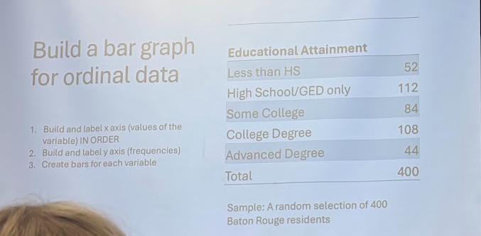
Build a bar graph for ordinal data
Build and label the x-axis (values of variable) IN ORDER
Build and label the y-axis (frequencies)
Create bars for each variable

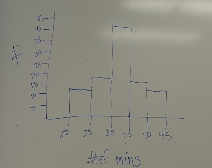
Histogram:
Bar graph for numerical variables (interval and ratio)
The bars are touching because numbers flow into each other (example: group age 20-29)
Values of the variable go on x-axis
Frequency goes on y-axis
Build a histogram:
Create a grouped interval frequency table with your data
X-axis: create tick marks across the bottom representing the lower or upper limits of your intervals. Label tick marks
Y-axis: create tick marks of equal distance for the frequencies up the y-axis. Label each tick mark. Be sure you can incorporate the highest frequency
Draw the bars for each interval (touching)
Label the graph with the variable name


Frequency distribution curve:
A distribution curve is a smooth graph that shows how often different values or ranges appear in a data set
X-axis: values
Y-axis: frequency
Interpreting frequency distributions:
Central location
Mean, Median, and/or mode
Spread (we’ll cover this soon)
Range and interquartile range
Standard Deviation and variance
Shape
Symmetry (evenness)
Modality (how many peaks)
Kurtosis (extreme values)
Distribution shapes
Normal distribution
Symmetrical
One mode
Mean, median, and mode are the same

Bimodal Distribution
Not a normal distribution (has more than one peak)

Uniform distribution
There is no shape/pattern to the distribution
Looks like a block/box

Skewed distributions
Look at the direction of the tail to determine skew
Left/negative skew
Right/positive skew
Skewed distributions and the mean:
When you have extreme high or low scores/data, it makes the mean an inaccurate representation of the data
The mean always goes towards the tail
If the mean is less than the median, it’s a left skew
If the mean is more than the median, it is a right skew
If they are close to each other, you have a normal curve
The median is the best measure of central tendency to use when you have skewed data


NEED TO KNOW MOST ABOUT SKEWED AND NORMAL DISTRIBUTIONS
Day 2
Research Q: On average, how many hours do college students sleep?
Survey Q: How many hours did you sleep last night?
Using the median for numerical data with skewed distribution
Symmetrical distribution (normal curve)
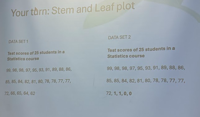
Test scores of 25 students in a stats course
99, 98, 98, 97, 95, 93, 91, 89, 88, 86, 85, 85, 84, 82, 81, 80, 78, 78, 77, 77, 72, 66, 65, 64, 62
Mean: 82.5 Median=84
Asymmetrical distribution (skewed curve)
Test scores of 25 students in stats course
99, 98, 98, 97, 95, 93, 91, 89, 88, 86, 85, 85, 84, 82, 81, 80, 78, 78, 77, 77, 72, 1,1,0,0
Mean: 72.6 Median: 84
How do I know if a distribution is skewed?
Pearson’s Median Skewness
Calculate mean minus the median
Multiply that difference by 3
Divide by the standard deviation
Assess the skewness
Greater than 1.0 (positive or negative) (ignore the negative sign ex. -1.125 is greater than 1.0)
Direction of skew
Positive number = right skew
Negative number = left skew
Example 1:
real estate prices
Mean: $450,000
Median: $380,000
Standard Deviation: $120,000
Calculation: [(450-380)*3]/120= 1.75
Is this data set skewed
Right positive skew
Example 2:
employee commute times
Mean: 28 min
Median: 31 min
Standard deviation: 8 min
Calculation: -1.125
Is this skewed:
Left negative skew because it is negative and it is over 1.0
Example 3:
Age of college students attending night school
Mean: 32
Median: 34
Standard deviation: 9
Calculation: -0.67
Is this skewed
There is no skew because 0.67 is less than 1
Stem and Leaf plot
Stem represents tens
Leaf represents ones
Ones have to be in perfect alignment (if turned sideways it would look like a histogram)
Need to have a key
Example: Key = 2 l 1 = 21
Benefits
preserves raw data
handy for small data set
spot outliers
shows the distribution shape
find quick statistics

Let’s create one:


Your turn:


Part 1 is the objective stuff (multiple choice/matching)
Part 2 is solving
Practice exam is almost identical to the actual exam just with different numbers
Practice exam is the best study tool