Lecture 8: Introduction to Spatial Statistics

I. Spatial Statistics

Quantify relationships or patterns
Compare geographical features
Track temporal changes

Traditional vs Spatial Statistics

Same objective: to understand the probability that a pattern actually exists VS random chance
Traditional statistics work with attribute values alone
- not accounting for the underlying spatial relationships that might exist in the datasets

Space is fundamental to spatial statistics

Location and spatial relationship
Patterns may exist at a given location (patterns in attribute space)
Space / geography is incorporated into the mathematics
- Proximity / Neighborhood
- First Law of Geography: “Everything is related to everything else, but near things are more related than distant things.”

Spatial Statistics

Location-based technique that involves methods for analyzing spatial distributions, patterns, processes, and relationships
geospatial data + statistics
find patterns > assess trends > make decisions / draw conclusions
Why is it important?
- The spatial visualization provided in GIS entices the user to rely solely on maps and visual comparison among maps for decision-making
  - Easy to give misleading impressions from the data
  - Several parametric and nonparametric models in spatial statistics provide objective, data-driven methods for quantifying trends and detecting patterns in spatial data
- The spatial analyses provided in GIS introduce variability and uncertainty into subsequent analyses and decisions
  - Buffering: when the size of the buffer can affect the analysis
  - Map overlay operations produce estimates which may or may not be sound and have uncertainty associated with them
  - Automatic “geoprocessing” with raster data when values in the cells are arithmetically added or averaged does not take into account error propagation.
- “When we analyze our data outside of their spatial context—when we remove space and time from our data—it’s like we’re only getting half the story. Things happen in space and time, and if we ignore that, our analysis is going to be incomplete. This is an important difference between traditional statistics and spatial statistics: traditional statistics often make the assumption that data are free of something called spatial autocorrelation.”
  - - Dr. Lauren Scott, ESRI expert on Spatial Statistics

II. Geographical Distribution

Central Feature
- Identifies the most centrally located feature
- Point that is the shortest distance to all other points in the dataset
Mean Center
- Identifies the geographic center / center of concentration for a set of features
- Creates a new feature (not in the dataset)
Median Center
- Identifies the location that minimizes the overall Euclidean distance to the features in a dataset
- More robust to any outliers
Linear DIrectional Mean
- Identifies the mean direction and orientation of the lines
Standard Distance
- Measures the degree of concentration / dispersion of the features around the geometric mean center
Directional Distribution (Standard Deviation Ellipse)
- To summarize the spatial characteristics of the geographical features: central tendency, dispersion, and directional trends

III. Spatial Autocorrelation

Recall

Degree of dependency
- Based on Tobler’s first law of geography: “Everything is related to everything else, but near things are more related than distant things.”
- It is the correlation of a variable with itself through space (only 1 variable is involved)
- Patterns may indicate that data are not independent of one another, violating the assumption of independence for some statistical tests

Spatial Autocorrelation

How are the features distributed?
What is the pattern created by the features?
Where are the clusters?
How do patterns and clusters of different variables compare to one another?

IV. Statistical Methods in GIS

Types of Statistical Methods
- Descriptive statistics
  - similar to traditional statistics (computing mean, std dev, etc); single, summery measures of a spatial distribution
- Spatial pattern analysis
  - Checking hotspots / cold spots (clustering / dispersion), outliers
  - Two types:
    - Global Statistics
      - identify and measure the pattern of the entire study area
      - do not indicate where specific patterns occur
    - Local Statistics
      - identify variation across the study area, focusing on individual features and relationships to nearby features (for specific areas of clustering)
- Identifying and measuring spatial relationships
  - use of regression / spatial regression methods to examine relationships and identifying factors significant to / promoting the spatial pattern
- Geostatistics
  - predictive modeling, interpolation methods using sample points; ideal for analyzing and predicting the values associated with nearly any kind of spatially continuous phenomena
  - outputs: probability surface, a prediction surface, or an error surface

Spatial Autocorrelation (Moran’s I)

based on feature location and feature values simultaneously
Two types:
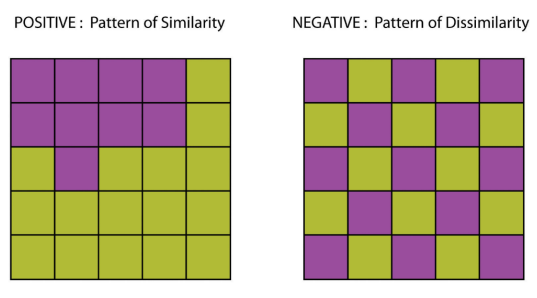
- Global Moran’s I: Measures whether the pattern of feature values is clustered, dispersed, or random
  - < 0: clustering of dissimilar values / values are dispersed
  - > 0: clustering of similar / values are clustered
  - 0: no autocorrelation / random distribution
- Local Moran’s I: Measures the strength of patterns for each specific feature. Compares the value of each feature in a pair to the mean value of all features in the study area.
  - > 0: feature is surrounded by features with similar values (either high or low); feature is part of a cluster
    - Statistically significant clusters can consist of high values (HH) or low values (LL)
  - < 0: feature is surrounded by features with dissimilar values; feature is an outlier
    - Statistically significant outliers can be a feature with a high value surrounded by features with low values (HL) or vice versa

Prediction with correlation and regression

Quantifying association or relationship of two (bivariate) or more (multivariate) attribute variables
Standard statistical models

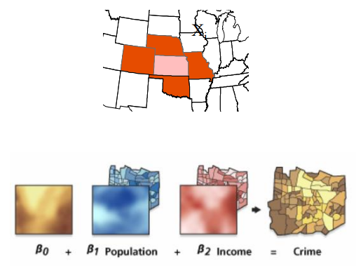
Spatial Regression (Geographically weighted regression (GWR))

local indicators applied to regression
calculates a separate regression for each polygon and its neighbors
maps the parameters from the model, such as the regression coefficient (b) and / or its significance value
Mathematically, this is done by applying the spatial weights matrix (W_ij) to the standard formulae for regression

Geostatistics

to analyse point data
to explore spatial variation in remote sensing data
to quantify noise in the images and for their filtering (e.g. filling of the voids / missing pixels)
to improve generation of DEMs
to optimize spatial sampling, selection of spatial resolution for image data and selection of support size for ground data
To predict values of a sampled variable over the whole area of interest
Prediction can imply both interpolation and extrapolation
Based on actual measurements and semi-automated algorithms

Interpolation Techniques

Deterministic techniques
- create surfaces from measured points based on either the:
  - extent of similarity (Inverse Distance Weighted) or
  - the degree of smoothing (Radial Basis Functions)
Geostatistical
- quantify the spatial autocorrelation among measured points and account for the spatial configuration of the sample points around the prediction location
  - Utilizes the statistical properties of the measured points (Kriging)
  - Kriging - geostatistical interpolation technique that estimates values at unmeasured locations based on known values at nearby locations, using a linear model that considers spatial autocorrelation

Examples and Applications

Geostatistical Mapping
Geostatistical Models