Introduction

When we understand the relationship between two variables, we can use the value of one variable to help us make predictions about the other variable.

3.1- Scatterplots and Correlation

Most statistical studies examine data on more than one variable. The analysis of multi-variable data builds on the foundation of single-variable processes.

When interpreting data:

• Plot the data, then add numerical summaries

• Look for overall patterns and departures from those patterns

• When there’s a regular overall pattern, use a simplified model to describe it

Explanatory and Response Variables

A response variable measures an outcome of a study. An explanatory variable may help explain or predict changes in a response variable. It’s easiest to identify explanatory and response variables when we specify values.

In many studies, the goal is to show that changes in one or more explanatory variables actually cause changes in a response variable.

Displaying Relationships: Scatterplots

The most useful graph for displaying the relationship between two variables is a scatterplot. The explanatory variable is plotted on the x-axis while the response variable is plotted on the y-axis. Because of this, the explanatory variable is usually referred to as x, and the response variable is referred to as y.

• A scatterplot shows the relationship between two quantitative variables measured on the same individuals. The values of one variable appear on the horizontal axis, and the values of the other variable appear on the vertical axis. Each individual in the data appears as a point in the graph.

How to Make a Scatterplot

1. Decide which variable should go on each axis

2. Label and scale your axes

3. Plot individual data values

Describing Scatterplots

To describe a scatterplot, follow the basic strategies of data analysis: look for patterns and important departures from those patterns.

How to Examine a Scatterplot

• You can describe the overall pattern of a scatterplot by the direction, form, and strength of the relationship

• An important kind of departure is an outlier, an individual value that falls outside the overall pattern of the relationship

Two variables have a positive association when above-average values of one tend to accompany above-average values of the other and when below-average values also tend to occur together.

Two variables have a negative association when above-average values of one tend to accompany below-average values of the other.

IMPORTANT: Not all relationships have a clear direction that we can describe as a positive or negative association.

Measuring Linear Association: Correlation

Linear relationships are particularly important because a straight line is a common pattern in scatterplots. A linear relationship is strong if the points lie close to a straight line and weak if they’re widely scattered about the line. Since our eyes aren’t good judges of how strong a linear relationship is, we use the numerical measure correlation (r) to supplement the graph.

• The correlation r measures the direction and strength of the linear relationship between two quantitative variables.

The correlation r is always a number between −1 and 1. Correlation indicates the direction of a linear relationship by its sign: r > 0 for a positive association and r < 0 for a negative association. Values of r near 0 indicate a very weak linear relationship. The strength of the linear relationship increases as r moves away from 0 toward either −1 or 1. The extreme values r = −1 and r = 1 occur only in the case of a perfect linear relationship, when the points lie exactly along a straight line.

Facts about Correlation

1. Correlation makes no distinction between explanatory and response variables

2. Because r uses the standardized values of the observations, r doesn’t change when we change the units of measurement of x, y, or both

3. The correlation itself has no unit of measure

Cautions to Keep in Mind When You Use Correlation

• Correlation doesn’t imply causation

• Correlation requires that both variables be quantitative

• Correlation only measures the strength of a linear relationship between two variables, never curved relationships

• A value of r close to 1 or −1 doesn’t guarantee a linear relationship between two variables

• Like mean and standard deviation, the correlation isn’t resistant: r is affected by outliers

• Correlation isn’t a complete summary of two-variable data, even when the relationship between the variables is linear

3.2- Least-Squares Regression

A regression line summarizes the relationship between two variables, but only when one of the variables helps explain or predict the other. Regression, unlike correlation, requires that we have an explanatory variable and a response variable.

• A regression line is a line that describes how a response variable y changes as an explanatory variable x changes. We often use a regression line to predict the value of y for a given value of x

Interpreting a Regression Line

A regression line is a model for the data, much like density curves. The equation gives a description of what the model tells us about the relationship between y and x.

• Suppose that y is a response variable and x is an explanatory variable. A regression line relating y to x has an equation of the form

  y = a + bx

  In this equation,

• y (actually y hat) is the predicted value of the response variable y for a given value of the explanatory variable x

• b is the slope, the amount by which y is predicted to change when x increases by one unit

Prediction

We can use a regression line to predict the response y-hat for a specific value of the explanatory variable. Extrapolation is the use of a regression line for prediction outside the interval of values of the explanatory variable x used to obtain the line. These predictions aren’t usually accurate.

Residuals and the Least-Squares Regression Line

In most cases, no line will pass exactly through all the points in a scatterplot. Because the line predicts the vertical y, the prediction errors are in the vertical direction. Therefore, a good regression line makes the vertical deviations of the points from the line as small as possible. A residual is the difference between an observed value of the response variable and the value predicted by the regression line.

• residual = observed y - predicted y

  = y - y-hat

The least-squares regression line of y on x is the line that makes the sum of the squared residuals as small as possible.

Determining Whether a Linear Model Is Appropriate: Residual Plots

Although residuals can be calculated from any model that’s fitted to the data, the residuals from the least-squares line have a special property. The mean of the least-squares residual is always 0. Because of this, the horizontal line at 0 on the residual plot helps to orient us. This “residual = 0” line corresponds to the regression line.

• A residual plot is a scatterplot of the residuals against the explanatory variable. Residual plots help us assess whether a linear model is appropriate

Examining residual plots

When an obvious curved pattern exists in a residual plot, the model we are using is not appropriate. When we use a line to model a linear association, there will be no leftover pattern in the residual plot, only random scatter.

How Well the Line Fits the Data: The Role of s and r^2 in Regression

The Standard Deviation of the Residuals

To assess how well the line fits all the data, we need to consider the residuals for each of the data points, not just one. Using these residuals, we can estimate the “typical” prediction error when using the least-squares regression line. To do this, we calculate the standard deviation of the residuals.

• If we use a least-squares line to predict the values of a response variable y from an explanatory variable x, the standard deviation of the residual, s, is given by

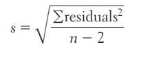
The Coefficient of Determination

The other numerical quantity that tells us how well the least-squares line predicts the values of the response variables is r^2, the coefficient of determination.

(for clarity purposes r^2 will be written as R-sq which is how some computer packages write it)

• The coefficient of determination is the fraction of the variation in the values of y that’s accounted for by the least-squares regression line

If all the points fall directly on the least-squares line, R-sq = 1.

Regression to the Mean

How to Calculate the Least-Squares Regression Line

From the data on the explanatory variable x and response variable, calculate the means x-bar and y-bar, and the standard deviations Sx and Sy of the variables and their correlation r. The least-squares regression line is the line y hat= a + bx.

When the variables are perfectly correlated, the change in the predicted response y hat is the same (in standard deviation units) as the change in x.

What happens if we standardize both variables?

Standardizing a variable converts its mean to 0 and its standard deviation to 1. This transforms the point (x-bar, y-bar) to (0, 0) so the line will pass through (0, 0).

Correlation and Regression Wisdom

1. The distinction between explanatory and response variables is important in regression.

2. Correlation and regression lines describe only linear relationships.

3. Correlation and least-squares regression lines are not resistant.

4. Association does not imply causation. A strong association between two variables is not enough to draw conclusions about cause and effect.

Outliers and influential observations in regression

• An outlier is an observation that lies outside the overall pattern. Points that are outliers in the y direction but not the x direction of a scatterplot have large residuals. Other outliers may not have large residuals.

• An observation is influential for a statistical calculation if removing it would change the results. Points that are outliers in the x direction of a scatterplot are often influential for the least-squares regression line.