Chapter 8

• Its average cost falls today because of economies of scale, and for any given level of output, its

average cost is lower in the next period due to learning by doing.

Top of Form

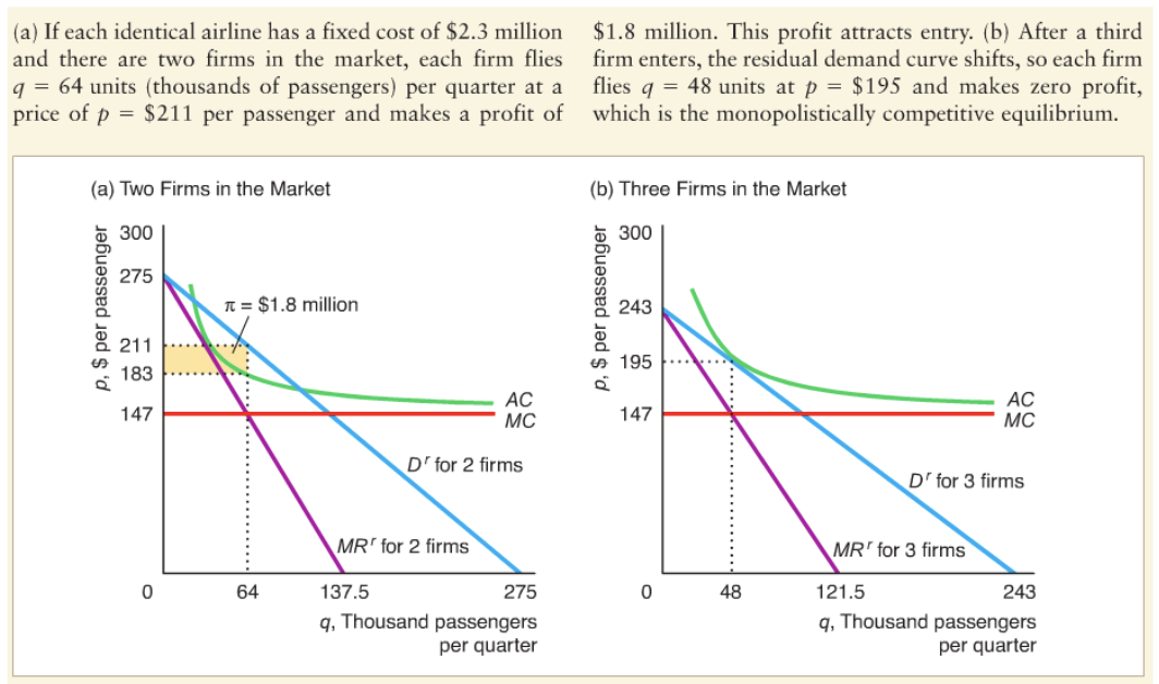
The way firms behave is influenced by the market's structure. This includes factors like the number of firms in the market, the ease of entering or exiting, and the extent to which firms can differentiate their products. These elements shape how firms make decisions about pricing, production levels etc.

In a competitive market, firms decide how much to produce to make the most profit. They weigh their costs and the demand in the market. Factors like the number of firms, how easy it is to join the market, and product uniqueness affect their choices (market structure). Firms producing similar goods can't charge higher prices than the market's price because consumers will choose cheaper options. So they focus on production decisions based on the market price, not on what other firms are doing.

8.1 Perfect competition

Price taking

In economics, a market is considered competitive when each firm within it is a "price taker." Price taker: Firms cannot really influence market prices for their goods or input costs, so they don’t set prices .

• Buyers and sellers , buy and sell at the market price

The reason behind this is the horizontal nature of their demand curve at the market price (elastic demand) . So, the firm has no control over the price it sells at because customers in the market are extremely sensitive to price changes. If the firm tries to increase the price, customers will stop buying altogether. And at the market price, the firm can sell however much it wants without affecting that price.

1. Many Small Buyers and Sellers: When there are numerous sellers in a market, no individual firm has the power to influence prices. The small size of each firm in comparison to the entire market ensures that its output has minimal impact on market price. Therefore, each firm can sell as much as it wants at the market price without

EX: There are thousands of small coffee shops in a city. Each shop sells coffee at the same market price and cannot affect the overall coffee price.

1. Identical Products: Firms in a perfectly competitive market sell identical products. Consumers do not differentiate between suppliers; they consider all goods as the same. This uniformity eliminates the ability of any individual firm to set a higher price.

Ex : Farmers sell wheat to a grain market. Wheat from one farmer is indistinguishable from that of another, so buyers don’t pay more for any specific farmer's wheat.

1. Full Information and Negligible Transaction Costs: Perfect competition assumes that all market participants have complete information about prices and products. Additionally, transaction costs are insignificant, facilitating easy and efficient transactions among buyers and sellers.

Ex : online auction sites like eBay, where buyers and sellers have access to complete product information and can trade easily, showcasing minimal transaction costs.

1. Free Entry and Exit: Firms can enter or exit the market without barriers. If one firm earns higher profits due to a price increase, other firms can enter the market, increasing supply and causing the price to fall back to its original level. Likewise, firms can exit the market without obstacles if profits decrease.

Ex : A new bakery can easily enter the market, but if profits decline due to competition, it can leave without any issues to avoid losses.

Derivaition from perfect competiton

In markets that don't have all the features of perfect competition (imperfectly competitive markets), buyers and sellers can still act as price takers. Even if there are some restrictions or not everyone has full information, these markets can still behave like competitive ones, making buyers and sellers respond to the market price without significantly impacting it.

Derivation of a Competitive Firm’s Demand Curve

Each firm faces what's known as a "residual demand curve," representing the demand left for that specific firm at different prices.

This residual demand curve {D’(p)} is derived by subtracting the supply from all other firms (market supply) from the overall market demand.

D’(p)= D(p)-S°(p)

EX : At p=$63, for example, the market demand is 527 units, but other firms supply only 434 units

• Market demand (D(p)) at $63 per chair = 527 units

• Supply of other firms (S°(p)) at $63 per chair = 434 units

• (Dr)/ D’(p) = 527 units - 434 units = 93 units

the elasticity of demand faced by a single firm (εi) in a market with n identical firms is

εi = nε - (n - 1)ηo

• ε is the market elasticity of demand (negative value).

• ηo is the elasticity of supply of the other firms (typically a positive value).

• n is the number of other identical firms in the market.

This equation suggests that a firm's residual demand curve becomes more elastic when:

1. There are more firms (n) in the market.

2. The market demand is more elastic (higher |ε|).

3. The elasticity of supply of the other firms (ηo) is larger.

Ex: In the Canadian metal chair manufacturing market, there are 78 firms. The elasticity of supply for the other firms (ηo​) is 3.1, and the elasticity of demand (ε) is -1.1. Assuming all firms in the market are identical, calculate the elasticity of demand facing a single firm in this market. Is the residual demand curve highly elastic?

εi​=nε−(n−1)ηo

(n) = 78 , (ηo​) = 3.1 , (ε) = -1.1

​εi​=[78×(−1.1)]−[77×3.1]

εi​=[−85.8]−[238.7]

εi​=−324.5

Why do we study perfect competition ?

• Understanding perfect competition helps economists predict how changes in taxes, costs, incomes, and other factors impact these actual markets.

• Economists use this model as an ideal benchmark to compare with real markets. Throughout the book, it's assumed that if a market differs from perfect competition, it might lead to societal problems.

8.2 Profit maximization

All firms not just competitive ones want to maximize their profit

• Many business people say so

• A firm that doesn’t maximize their profit will probably lose money and lose their business.

Profit: Profit is what a business earns after subtracting its costs from its revenue. {R-C}

Revenue: product of price x quantity sold. {P x Q}

It’s hard to measure costs, economists measure of costs is “opportunity cost”/ “economic cost”

Economic profit: Revenue – opportunity cost

Business Profit vs. Economic Profit: Business profit only considers explicit costs (like wages and materials) but ignores opportunity costs (the value of the best alternative use of resources). Economic profit includes both explicit and opportunity costs.

Ex: Let's say you run your own business and make a business profit of $20,000 per year. However, the economists highlight that your economic profit might be lower if you could have earned $25,000 annually working elsewhere. Your economic profit is actually a loss of $5,000 because you forewent a higher salary.

Ignoring opportunity cost might lead to a mistaken conclusion that your business is profitable when, it's actually less beneficial than other options. So, economic profit, considering all opportunity costs, provides a clearer understanding of the actual gains or losses from a business or investment.

Ex : investing in something should only happen if it yields more profit than the best alternative use of funds, like earning interest in a bank.

Two decsions to maximizing profit

A firm's profit, π, is revenue (R) minus cost (C). Profit can be positive (a gain), zero (break-even), or negative (a loss).

To maximize profit, firms consider two decisions:

• Output Decision: Determine the level of output (q*) that maximizes profit.

• Shutdown Decision: Choose whether to produce q* or shut down to reduce losses.

1. Output Decision Rules:

• Output Rule 1: Produce at the output where profit is maximized.

• Output Rule 2: Set output where marginal profit (additional profit from one more unit) is zero.

Marginal profit (q)= MR(q)-MC(q)

MR(q)=MC(q)

• Output Rule 3: Choose output where marginal revenue equals marginal cost (MR = MC).

1. Shutdown Decision Rule:

• Rule 1: A firm should shut down only if it can reduce its loss by doing so, not simply if it's making a loss.

• In the short run, firms weigh variable costs against revenue to decide whether to stop operating. Fixed costs (like equipment) that are sunk (already incurred and cannot be recovered) are irrelevant to this decision.

• If revenue covers variable costs but is less than total costs (variable plus avoidable fixed costs), the firm may continue operations to offset some fixed costs.

• Short-run decisions assume fixed costs are sunk; they pay this cost whether operating or not.

• Rule 2 : firms shuts down only if it’s revenue is less than it’s avoidable cost.

• Rule 3: shutdown if price falls between the minimum of the AVC curve (shutdown point)

8.3 Competition in the short run

In economics, the short run is a period where at least one input (like capital or machinery) is fixed and cannot be changed quickly.

• Due to fixed inputs, new firms can't enter the market, and existing firms can't fully exit or alter their capital in the short run.

Firms in the short run aim to maximize profit or minimize losses given their fixed inputs.

They decide the level of output hat best aligns with their profit goals, considering their fixed resources.

Short-run output decision

• Competitive firms aim to maximize profit in the short run.

• A competitive firm's marginal revenue equals the market price because it can sell all units at that price.

MC(q)= p.

• To maximize profit, the firm produces where marginal cost equals the market price:

Ex :

p - AC

The firm's profit per unit is the difference between the market price and average cost: Profit per unit = Market price−Average cost

Short-run shutdown decsion

• Firms decide to shut down only if doing so reduces their loss.

• A competitive firm shuts down if its revenue is less than its avoidable variable cost: R(q) < VC(q) or, equivalently, if the market price is less than short-run average variable cost: p < AVC(q).

• Bottom of FormEx : If the market price is above the firm's average cost at the produced quantity, it makes a profit and continues operating.

• If the market price falls below the average cost but remains above the average variable cost, the firm should continue operating in the short run.

• If the market price exceeds the minimum average cost ($6 in the lime firm example) at the produced quantity, the firm makes a profit and keeps operating.

• If the market price is between the minimum average cost and the minimum average variable cost, the firm operates even if it incurs a loss because shutting down would increase the loss.

• However, if the market price drops below the minimum average variable cost, the firm should shut down because it would suffer a greater loss by operating compared to shutting down.

Short-Run Firm Supply Curve for a Competitive Firm:

• A competitive firm's supply curve in the short run is determined by its marginal cost curve above its minimum average variable cost (AVC).

• The supply curve traces the firm's output levels at different market prices.

• When the market price is above the minimum AVC (for example, above $5 in the lime firm example), the firm's supply curve mirrors its marginal cost curve.

• However, if the market price falls below the minimum AVC (below $5 in the lime firm example), the firm doesn't supply any output, i.e., it shuts down and produces zero.

• A competitive firm's short-run supply curve is how much it's willing to produce at different prices in the short term.

• It matches the firm's costs:

  • If the price is higher than what it costs to make something (more than the minimum average cost of making it), the firm will supply more.

  • But if the price is too low (below what it costs to make it), the firm won’t produce anything in the short term.

• This curve indicates how much the firm will produce at different prices if it covers its basic costs.

• Top of Form

Bottom of Form

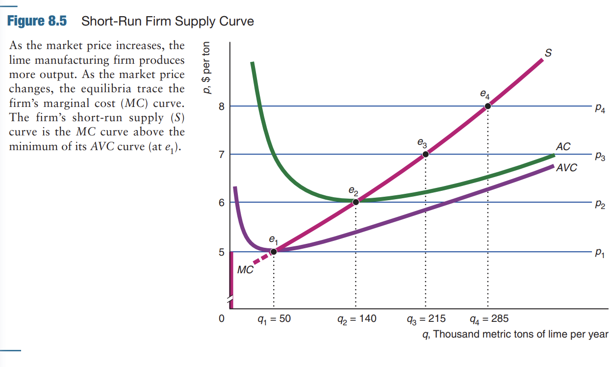• As the market price increases from $5 to $8, the lime firm's output also increases accordingly (from 50 to 285 thousand tons per year).

• Each equilibrium point (e1 to e4) in the graph represents the intersection of the market price line and the firm's marginal cost curve, determining the profit-maximizing output for each price.

• The short-run supply curve, represented by a solid red line, matches the firm's marginal cost curve when prices are above the minimum AVC, showcasing the output the firm is willing to supply at different market prices.

Short-run competitive equilibrium

The combination of the short run market supply curve and the market demand curve gives the short run competitive equilibrium.

• when supply and demand balance in the short term in a market.

8.4. competition in long run

Long-run compeptitive profit maximization

In the long run, firms have the flexibility to adjust all of their inputs, including capital and production scale.

1. Output Decision: The firm aims to maximize its profit by producing the quantity where long-run marginal profit is zero or where long-run marginal cost equals marginal revenue.

2. Shut Down Decision: Once the firm determines the output level that maximizes its profit, it evaluates whether it should produce or shut down. The firm will shut down if its revenue is less than its avoidable cost. In the long run, all costs are variable, so the firm considers shutting down if operating at the determined output level would result in an economic loss.

Long run firm supply curve

For a competitive firm, the long-run supply curve is represented by its long-run marginal cost curve above the point where the market price exceeds the minimum of its long-run average cost curve. This curve indicates the various quantities of output the firm is willing to supply at different market prices in the long run.

In the long run, a competitive firm won't operate at a loss. If the market price falls below the firm's minimum long-run average cost, such as $24 in this example, the firm will choose to shut down rather than continue operating at a loss.

The long-run supply curve of a competitive firm depends on its long-term production costs compared to market prices. It's based on the firm's ability to adjust and produce more when the market price is higher than its lowest long-term average cost. This curve shows how much a firm will supply at different prices, considering its costs and profit goals in the long run.

Long run market curve

1. Entry and Exit in the Long Run: Firms decide to enter a market if they can make a long-term profit and exit if they face long-term losses. If firms are making zero long-term profit, they tend to stay in the market.

The supply curve is horrizontam at the minimum LR AC

1. Long-Run Market Supply with Identical Firms and Free Entry: In a situation where an unlimited number of firms have the same costs and can freely enter and exit, the long-run market supply curve is flat at the minimum long-run average cost. Firms enter when the price is above this minimum cost, expanding market output until profit is driven to zero.

2. Limited entry : The LR market curves slopes upward

Market’s limited if , the gov restricts the market entry, entry price is high and scarce resources

1. Firms cost fct differ: LR curve slopes upwards, only if the lower-cost firms can produce as much output as the market wants., firms with low minimum AC, are willing to enter the market at lower prices than others

2. Effect of Input Prices on Market Supply (limited entry): If input prices rise with market output, the long-run supply curve slopes upward. This situation occurs in markets where the demand for inputs increases as the market output expands, causing a rise in the marginal cost of production.

3. Impact of a Large Buyer: When a significant buyer, like a country in a global market, demands a substantial portion of a good, the residual supply curve faced by that buyer can vary. A country importing a small fraction of the world's output might face a nearly horizontal residual supply curve, while a large consumer may encounter an upward-sloping residual supply curve. This curve reflects the quantity the market supplies that is not consumed by other demanders at any given price.

The residual supply curve: the QT the market supplies that’s not consumed by other demanders at any given price. (=excess)

Chapter 9

Long-run competitive equilibrium: the intersection of the long-run market supply and demand curves

How can we use the competitive market model to answer these questions:

• How does a competitive model can predict how changes in government policies (ex: taxes on imports, import quotas, global warming) affect consumers and producers. 

• We will examine the properties of a competitive market and how government actions and other shocks affect the market and its properties. 

• The two main properties we will see of a competitive market.  

  1. Firms in a competitive equilibrium generally make zero (economic) profit in the long run.  

  2. Competition maximizes a measure of societal welfare. 

General definition: Welfare is when the government’s payments to poor people.  

In economics :  Welfare is the well-being of society. 

 Remember:  

• Consumer surplus is also called consumer welfare  

• Producer surplus is also called producer welfare.  

Welfare economics: is the study of the impact of a change on various groups’ well-being. 

Thanks to this study, economists can advise policymakers on  

• who will benefit 

• who will lose 

• what the net effect of this policy will likely be. 

9.1: Zero Profit for Competitive Firms in the Long Run: 

In a perfect competition market firms  

• Earn zero profit in the long run  

• Must maximize profit. 

Zero Long-Run Profit with Free Entry: 

In the long-run, supply curve is horizontal if firms  

• Are free to enter the market 

• Have identical cost 

• Input prices are constant.  

• Operate at minimum long-run average cost —> they are indifferent between shutting down or not because they earn zero profit. 

Rappel: 

Economic profit: Revenue - opportunity cost.  

opportunity cost: is the opportunity you lose while doing something else. 

The difference between economic profit and business profit (accounting profit) :  

Accounting Profit: its the financial gain or loss calculated by subtracting the explicit costs from total revenue.( its the profit you will see in your accounting)   

Economic Profit: it takes into account both explicit costs and implicit costs (opportunity costs). It measures the true economic gain or loss by considering the value of resources used in the business, including the potential earnings foregone in the next best alternative. 

 Because business cost does not include all opportunity costs, business profit is larger than economic profit. Thus, a profit-maximizing firm may stay in business if it earns zero long-run economic profit, but it shuts down if it earns zero long-run business profit. 

Zero Long-Run Profit When Entry Is Limited 

One of the reasons why there a limited number of firms in the market is due to the limitation of the supply of an input. And this is the reason why firms earn zero profit —> they are linked with the scarcity of input which puts its price up until the firms’ profits are zero. 

Ex: there’s a limitation in land to produced potato’s, since potato’s are rare it’s price is going to rise cause the owners profit to decrease until zero  

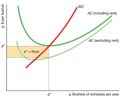
“π” represents the opportunity cost. The rent is thus a fixed cost to the farmer because it doesn’t vary with the amount of output. It affects just the AC but not the MC.  

• As a result, if the owner produces at all, he will produces at q* where its marginal cost equals the market price.  The minimum point of the AC is p* at q* —> zero economic profit. Even with a shift of the market price the situation will equilibrate itself. 

Rent: its the payment made to use or access an input and it goes to the owner of that input. 

Ex: land, property, or equipment 

If firms are making economic profits in the short run due to a scarce input, it causes that the market price for the goods or services they produce is high enough to cover their variable costs and contribute to a positive economic profit. 

Three things happens 

1. Consumers want more of the product so the demand shift to the right causing the price to increase 

2. When other firms observe these economic profits, they will enter the market to also have some profits causing the supply curve to shift to the right (more quantity supplied).  

3. If the supply increase, the prices of the good will go down. Making the economic profit back to zero AGAINE 

In the long run, firms continue to enter the market as long as there is an economic profit to be made, but as more firms enter, the supply keeps increasing bringing the prices down. This process continues until the price settles at a level where all firms earn zero economic profit. 

The long-run equilibrium in a perfectly competitive market is characterised by firms earning zero economic profit, meaning that they can cover all of their costs, (opportunity cost and explicit cost). This situation occurs when the market price settles at the minimum point on the long-run average cost curve. 

The Need to Maximize Profit 

In a competitive market with identical firms and free entry the key to survive is to maximise its profit. 

 9.2 Consumer Welfare 

Economists and policymakers want to know how much consumers benefit from or are harmed by shocks that affect the equilibrium price and quantity. To what extent are consumers harmed if a local government imposes a sales tax to raise additional revenues? To answer such a question, we need some way to measure consumers’ welfare. 

If we knew a consumer’s utility function, we could directly answer the question of how an event affects a consumer’s welfare. If the price of beef increases, the budget line facing someone who eats beef rotates inward, so the consumer is on a lower indifference curve at the new equilibrium.  

But this technic is not appropriate because  

1. We rarely, know the utility functions of individuals .  

2. Even if we had the utility function of multiple consumers, we wouldn’t be able to compare them. One person might say that he got 1,000 utils from the same bundle that another consumer says gives her 872 utils of pleasure. It’s not relevant because they just might be using a different scale  

CCL: we measure consumer welfare in terms of dollars. 

Measuring Consumer Welfare Using a Demand Curve 

Consumer welfare from a good is the benefit a consumer gets from consuming that good minus what the consumer paid to buy the good. 

Generally, you buy things that are worth more to you than what they cost. Imagine that you are very thirsty. You can buy a soft drink for $1, but you’d be willing to pay much more because you are so thirsty. 

If we can measure how much more you’d be willing to pay than what you did pay, we’d know how much you gained from this transaction and the demand curve contains the information we need to make this measurement. 

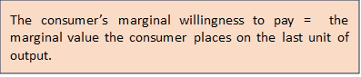
Marginal Willingness to Pay: To measure the welfare we need to know that the demand curve reflects a consumer’s marginal willingness to pay: the maximum amount a consumer will spend for an extra unit of a good. 

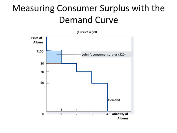
Johns demand curve for magazines per week, indicates his marginal willingness to pay for various numbers of albums. John places a marginal value of $100 on the first album, $80 on the second album…... As a result, if the price of an album is $5, John buys one album. If the price is $80, he buys two albums……  

Johns consumer surplus is his marginal willingness to pay minus what he pays to obtain the magazine

Consumer Surplus: The difference between what a consumer is willing to pay for the quantity of the good purchased and what the good actually costs. 

Consumer surplus is a measure of the extra pleasure the consumer receives from the transaction beyond its price. 

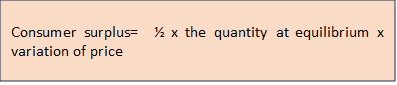
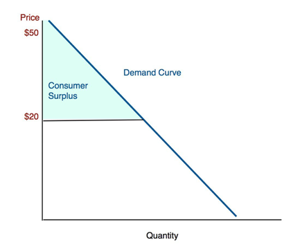Consumer surplus (CS) , is the area under the demand curve and above the horizontal line at the price p* up to the quantity he buys, q*.

• We can measure the consumer surplus for 1 individual using his individual demand curve but we can also do the same with all consumers in a market using the market demand curve. Market consumer surplus is the area under the market demand curve above the market price up to the quantity consumers buy. 

Effect of a Price Change on Consumer Surplus 

If the supply curve shifts upward or a government imposes a new sales tax, the equilibrium price rises, reducing consumer surplus.  

• In general, remember that when the price increases, consumer surplus falls ( they have less deals, they are less willing to spend ) causing the demand curve to be less elastic. 

• When the price decrease, consumer surplus increase ( they will have more deals, they are more willing to spend) causing the demand curve to be more elastic.  

Consumers would benefit if policymakers, before imposing a tax, considered in which market the tax is likely to harm consumers the most. 

9.3: Producer Welfare:  

Producer surplus (PS); is the difference between the amount for which a good sells and the minimum amount necessary for the seller to be willing to produce the good. (It’s the supplier’s gain from participating in the market)   

Remember: The minimum amount a seller must receive to be willing to produce is the firm’s avoidable production cost.  

 Measuring Producer Surplus Using a Supply Curve:  

To determine a competitive firm’s producer surplus, we use its supply curve:  

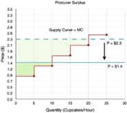• Its marginal cost curve above its minimum average variable cost. 

• Variable cost of producing four units: sum of the marginal costs for the first four units:  VC = MC1+ MC2+ MC3+ MC40 

• The firm’s total producer surplus, PS, from selling four units at $4 each is the sum of its producer surplus on these four units:  PS = PS 1 + PS2 + PS3+ PS  4 —>$3 + $2 + $1 +$0 = $6 

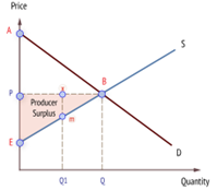Graphically : Producer surplus is the area above the supply curve and below the market price up to the quantity produced. The variable cost for all the firms in the mar- ket of producing Q is the area under the supply curve between 0 and the market output, Q. 

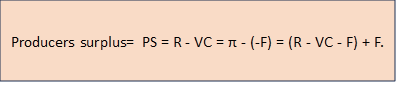
• Difference between producer surplus and profit the fixed cost:  

 F = PS – π =  

PS = (R - VC)   

Profit = R— C  but C = VC— F so profit = R — VC — F   

CCL = profit = R –VC —  (R – VC - F) = F 

If F = 0 (as often occurs in the long - run), producer surplus = profit 

Another interpretation of producer surplus is as a gain to trade. 

In the short - run:  

• If the firm produces and sells its good,  trades, the owner earns a profit. (of R - VC - F.)  

• If the firm shuts down, they don’t trade anymore, the owner doesn’t loses its fixed cost of ( — F) 

So producer surplus equals the profit  minus the profit (loss) from not trading 

 Using Producer Surplus 

Imagine you have a bunch of companies that make and sell a product, like ice cream. Now, producer surplus is like the extra money these companies make beyond covering their costs. It's a measure of how much they gain from selling their products. 

Now, let's say something changes, like the price of sugar (an ingredient for the ice cream) goes up. This is a shock to the market.. 

Consequences :   

• The effect on all firms: Producer surplus helps us figure out how much all the ice cream companies together are affected by this change. We don't need to check each company's profit individually. 

• Market producer surplus: We can use the idea of producer surplus to calculate the overall impact on the entire ice cream market, just like we would have done for one company. It's a way of looking at the big picture. 

• Fixed costs don’t change: If the change (like the sugar price increase) doesn't affect the fixed costs of running an ice cream company (like rent for the factory), then the change in profit is exactly the same as the change in producer surplus. So, if the companies collectively make more money (or less) due to the sugar price change, that's also the change in their profit. 

Thanks to producer surplus we can quickly see how all the companies in a market are impacted by changes, without getting into the details of each company's finances.  

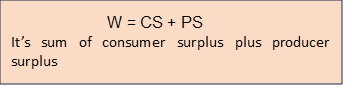
9.4 : Competition Maximizes Welfare :  

 Remember that welfare is the study of the impact of a change on various groups’ well-being. Generally in economics we can conclude that it’s the well-being of society 

Using this measure, we make a value judgment that the well-being of consumers and producers equally important. 

One of the most IMPORTANT results in economics is that competitive markets maximise this measure of welfare. If either less or more output than the competitive level is produced, welfare falls. 

• Consumer Surplus: This is the benefit consumers receive because they are paying less for a product than the maximum price they are willing to pay. 

• Producer Surplus: On the other side, producers (smartphone manufacturers in this case) gain surplus because they are selling the smartphones for more than the minimum price they are willing to accept. 

In a perfectly competitive market, the forces of supply and demand determine the equilibrium price and quantity. This equilibrium represents the most efficient allocation of resources, maximizing the combined consumer and producer surplus. If the market produces less than or more than this equilibrium quantity, welfare (the sum of consumer and producer surplus) decreases. 

Example: 

Case 1 - Below Equilibrium Quantity: Let's say the market produces fewer smartphones than the equilibrium quantity. Consumers who are willing to pay more for a smartphone at the equilibrium price can't find enough of them. This reduces consumer surplus. Meanwhile, producers are not selling as many smartphones as they could at the equilibrium price, decreasing producer surplus. 

Case 2 - Above Equilibrium Quantity: If the market produces more smartphones than the equilibrium quantity, consumers may pay less for each smartphone, but now there are more smartphones than consumers are willing to buy at that price. This results in a reduction of consumer surplus. Additionally, producers have to lower prices to sell the excess smartphones, reducing their surplus. 

In both cases, the combined consumer and producer surplus is reduced compared to the situation where the market is at the equilibrium quantity. This is why economists often emphasize that competitive markets, when left to operate freely, tend to maximize overall welfare. Any deviation from the equilibrium quantity tends to reduce this overall welfare. 

NB: Not everyone agrees that society should try to maximize this measure of welfare, some argue that only CS or only PS should be included. If there’s either less or more output than the competitive level is produced, welfare falls.  

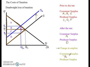
Deadweight loss: net reduction in welfare from a loss of surplus by one group that is not offset by a gain to another group from an action that alters a market equilibrium.  

Society would be better off producing and consuming extra unit of this good than spending this amount on other goods. The deadweight loss is the opportunity cost of giving up some of this good to buy more of another good. It reflects a market failure, inefficient production or consumption, often because a price exceeds marginal cost 

9.5 Policies That Shift Supply and Demand Curves:  

Economists have developed welfare tools to predict the impact of government programs that alter a competitive equilibrium.  

Note that all governmental actions affect a competitive equilibrium in many ways.  

1. Some it shifts the demand curve or the supply curve.  

Ex: a limit on the number of firms in a market.  

1. Some create a wedge or gap between price and marginal cost so that they are not equal, even though they were in the original competitive equilibrium.  

Ex: sales taxes 

3. It moves us from an unconstrained competitive equilibrium to a new, constrained competitive equilibrium.  

(Information note: governmental policies can cause the supply curve or the demand curve to shift, be in this course we will only concentrate on policies that limit supply because they are used more frequently and have clear effects) 

If a government policy causes the supply curve to shift to the left, consumers make fewer purchases at a higher price and welfare falls.  

(Ex: here the original consumer surplus is A + B + E and welfare was equal to A + B + E + C + D + F . After the governmental policy the supply shift to the left and the new price equilibrium is P2, the new consumer surplus falls to A and welfare falls to A + B + C.)  

The only “trick” is that we use the original supply curve to evaluate the effects on producer surplus and welfare 

Example of ways government force the supply to shift to the left:  

Restricting the number of firms in a market —> licensing taxicabs, psychiatric hospitals, or liquor licenses.  

Entry Barrier: (raising the cost of entry in the market). If the cost of entering is greater than  firms already in the market, a potential firm might not enter a market even if existing firms are making a profit. This restriction is only applied to new firm wanting to enter the market, it discourages them. Current firms in the market do not bear the cost.  

It discourages them because at the time they entered the market they also have other cost to pay such as the fixed costs of building plants, buying equipment, and advertising a new product. But if new firms see that current firms in the market have to pay the same cost as them and if in addition, they see that they are still making profit they won’t be discourage, they know that they will do as well as existing firms once they begin operations, so they are willing to enter as long as profit opportunities exist. 

Large sunk costs can be barriers to entry under two conditions:  

1. If *capital markets do not work efficiently so that new firms have difficulty raising money, new firms may be unable to enter profitable markets.

*Capital markets are places where people buy and sell long-term investments like stocks and bonds (la bourse).  

1. If a firm must incur a large sunk cost, which increases the loss if it exits, the firm may be reluctant to enter a market in which it is uncertain of success. 

Exit Restriction: some laws that delay how quickly some firms may go out of business so that workers can receive advance warning that they will be laid off).  

• In the short run: these restrictions keep the number of firms in a market high.   

• In the long run: they may reduce the number of firms in a market.  

Why do exit restrictions reduce the number of firms in a market in the long run? :  

Imagine your firm’s only input is labor. You know that at a certain moment you will have less demand from consumers (during business slowdown or winter for example). During this period, to avoid additional cost such as paying your workers, it’s more beneficial for you to shut down. You enter this market if you expect your economic profits during good periods to be zero or positive. 

(When exit restriction comes in) A law that requires you to give your workers six months’ warning before firing them, prevents your firm from shutting down quickly causing you to suffer losses during business downturns since you’ll have to pay them for six months even if you have nothing for them to do.  

With full knowledge of the facts you are less willing to enter the market. Unless the economic profits during good periods are much high enough to compensate your losses, you will not choose to enter the market.  

Ccl: If exit barriers limit the number of firms, cause prices increase, lower consumer surplus, and reduce welfare. 

 9.6 Policies That Create a Wedge Between Supply and Demand :  

The most common government policies that create a wedge between supply and demand curves are sales taxes (or subsidies) and price controls.  

These policies create:  

- a gap between marginal cost and price   

- the market to produces either too little or too much.  

Explanation: 

Imagine the cost of making your toy is like the price tag on it, and you and your friends have a certain amount you're willing to pay for it. When the government adds a tax, you have to pay a little extra. So, the price becomes more than what it costs  to make the toy. (Ccl: due to a tax it causes the price of the good to exceed marginal cost).  

The price is higher than what you all think the toy is worth you might not want to buy as many toys as before . So, even though you'd like to buy more and the seller would like to sell more, the higher price makes everyone a bit unhappy causing consumer surplus, producer surplus, and welfare to fall 

Another example:  

If the government says the price has to be lower than what it costs to make the toy, it might seem great because it's cheaper, but the seller might not want to make as many because they're not making enough money (profit). So, even though you'd like to buy more, there might not be enough toys . 

That's why we say that this policies causes a "wedge" between what people want to do and what the government rules make them do. 

Welfare Effects of a Sales Tax:  

A new sales tax causes  

• The price consumers pay to rise, resulting to a loss of consumer surplus, ∆CS .  

• A fall in the price firms receive, resulting in a loss of producer surplus, ∆PS 

However, the new tax provides the government with new tax revenue, ∆T = T  

In the case where the government does something useful with the tax revenue, this is the new formula for welfare: 

As a result, the change in welfare is