Chapter 13: F Distribution and One-way Anova

Analysis of Variance: For hypothesis tests comparing averages between more than two groups

ANOVA Test: determine the existence of a statistically significant difference among several group means.
Variances: helps determine if the means are equal or not
ANOVA Conditions
- Each population from which a sample is taken is assumed to be normal.
- All samples are randomly selected and independent.
- The populations are assumed to have equal standard deviations (or variances).
- The factor is a categorical variable.
- The response is a numerical variable.
Ho: μ1 = μ2 = μ3 = … = μk
Ha: At least two of the group means μ1, μ2, μ3, …, μk are not equal. That is, μi ≠ μj for some i ≠ j.
The null hypothesis: is simply that all the group population means are the same.
The alternative hypothesis: is that at least one pair of means is different.
Ho is true: All means are the same; the differences are due to random variation.
Ho is NOT true: All means are not the same; the differences are too large to be due to random variation.

F-distribution: theoretical distribution that compares two populations
There are two sets of degrees of freedom; one for the numerator and one for the denominator.
To calculate the F ratio, two estimates of the variance are made.
1. Variance between samples: An estimate of σ2 that is the variance of the sample means multiplied by n (when the sample sizes are the same.).
2. Variance within samples: An estimate of σ2 that is the average of the sample variances (also known as a pooled variance).
  1. SSbetween: the sum of squares that represents the variation among the different samples
  2. SSwithin: the sum of squares that represents the variation within samples that is due to chance.
MS means: "mean square."
MSbetween: is the variance between groups
MSwithin: is the variance within groups.

k: the number of different groups
nj: the size of the jth group
sj: the sum of the values in the jth group
n: total number of all the values combined (total sample size: ∑nj)
x: one value→ ∑x = ∑sj
Sum of squares of all values from every group combined: ∑x2
Between-group variability: SStotal = ∑x2 – (∑𝑥2) / n
Total sum of squares: ∑*x^*2 – (∑𝑥)^2n / n
Explained variation: sum of squares representing variation among the different samples→ SSbetween = ∑[(𝑠𝑗)^2 / 𝑛𝑗]−(∑𝑠𝑗)^2 / 𝑛
Unexplained variation: sum of squares representing variation within samples due to chance→ 𝑆𝑆within = 𝑆𝑆total – 𝑆𝑆between
df**'s for different groups (df's for the numerator)**: df = k – 1
dfwithin = n – k*:* Equation for errors within samples (df's for the denominator)
MSbetween = 𝑆𝑆between / 𝑑𝑓between: Mean square (variance estimate) explained by the different groups
MSwithin = 𝑆𝑆within / 𝑑𝑓within: Mean square (variance estimate) that is due to chance (unexplained)
Null hypothesis is true: MSbetween and MSwithin should both estimate the same value.
The alternate hypothesis: at least two of the sample groups come from populations with different normal distributions.
The null hypothesis: all groups are samples from populations having the same normal distribution

Here are some facts about the F distribution.
- The curve is not symmetrical but skewed to the right.
- There is a different curve for each set of dfs.
- The F statistic is greater than or equal to zero.
- As the degrees of freedom for the numerator and for the denominator get larger, the curve approximates the normal.

In order to perform a F test of two variances, it is important that the following are true:
- The populations from which the two samples are drawn are normally distributed.
- The two populations are independent of each other.
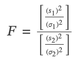
F has the distribution F ~ F(n1 – 1, n2 – 1)
where n1 – 1 are the degrees of freedom for the numerator and n2 – 1 are the degrees of freedom for the denominator.
F is close to one: the evidence favors the null hypothesis (the two population variances are equal)
F is much larger than one: then the evidence is against the null hypothesis
A test of two variances may be left, right, or two-tailed.
Examples