Module 2: One-Way ANOVA

Comparing Groups

The goal of comparing groups is trying to explain differences. To compare groups you have to first assemble groups, based on their preexisting characteristic (quasi-experimental), or based on the intervention that is going to be administered to them (experimental).

When trying to explain differences it is crucial to answer the following questions:

Does this grouping make sense?

Is this difference meaningful?

Confidence Interval: usually set to 95%; is a range where the true answer is in 95% of chances

Null Hypothesis Significance Testing: What is the probability that we would observe a difference of this magnitude if there was no real difference? - Egon Pearson, Jerzy Newman

The t-test: Comparing Two Groups

The t-test compares two means. Its main purpose is to test whether two group means are significantly different from one another

Between-groups: two experimental conditions participants were assigned to; sometime s called independent-samples, independent-measures, independent-means

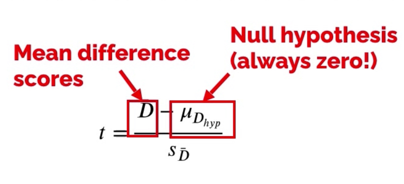
Repeated-measures: two experimental conditions, but the same participants took part in each condition; otherwise called paired-samples, dependent-means, matched-pairs

Standard Deviation (SD): measures how spread out the dataset is

Standard Error (SE): measure s how much the sample mean is expected to vary if we took multiple samples; a smaller SE means a more reliable estimate of the true population mean

Reliability = Consistency = Precision: how consistent measures are even if not correct

Validity = Accuracy: how close the measurement is to the true or correct value; the extent to which we are measuring the thing we want to measure

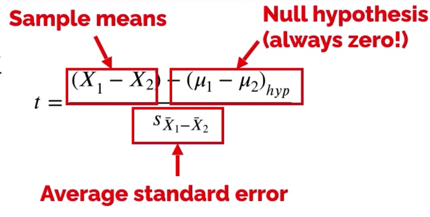
How the t-statistic works?

1. Two sample means are calculated

2. Under the null hypothesis we expect those means to be roughly equal

3. We compare the obtained mean difference against the null hypothesis

4. We use the standard error as a gauge of the random variability expected between sample means - if the difference is in the range of SE, the null hypothesis is accepted

5. If the difference between sample means is larger than expected based on the standard error:

   1. There is no effect and this difference occurred by chance

   2. There is an effect and the means are meaningfully different

The t-statistic assumptions:

• In the independent-samples:

  • Level of measurement (DV interval or ratio)

  • Random sampling

  • Normality

  • Homogeneity of variance

• In the repeated measures:

  • Level of measurement (DV interval or ratio)

  • Random sampling

  • Normality

  • NO homogeneity of variance because same individuals

The main problem with the t-test is that it can only compare two groups. If theres more groups to compare, an ANOVA test will suit better.

One-Way ANOVA: Comparing Three and More Groups

Type I Error: false positive - we say there is an effect when there is not one

Type II Error: false negative - we say there is no effect when there is one (Two blind to see an effect)

Why do we not do multiple t-tests?

Familywise Error Rate (FWER): The probability of making at least one Type I error (false positive) when performing multiple statistical tests. FWER controls the overall risk of incorrectly rejecting any true null hypothesis across a family of tests, ensuring the error rate remains at a desired level (commonly 5%) despite multiple comparisons.

• When conducting multiple t-tests, with each additional test the likelihood of Type I error jumps up. Although FWER can help account for that, using ANOVA instead completely eliminates the need for this hassle.

ANOVA

For ANOVA, the Null Hypothesis states that all of the population means are exactly the same - no significant difference between the means (H₀: μ₁ = μ₂ = … = μ_k); the Alternative Hypothesis states that at least one group is different from another.

ANOVA produces an F-statistic/ratio, which represents the ratio of the model (conditioned groupings) to its error.

ANOVA is an omnibus test, which means that it tests for an overall experimental effect. Significant F-statistic tells us that there is a difference somewhere between the groups, but not where the difference is.

Here is another way to explain how the One-Way ANOVA works. The total variance consists of the between-conditions driven variability (the model; the actual differences between conditions), and within-conditions driven variability (the error; like preexisting differences). ANOVA compares these two variabilities and finds out which is more prevalent.

The F-test divides the between-conditions variability by the within-conditions variability. Between group variability consists of the random error and treatment effect. If the treatment effect is 0, the F-value is going to be 1 (Null Hypothesis accepted). However, as the treatment effect increases, the F-value increases as well.

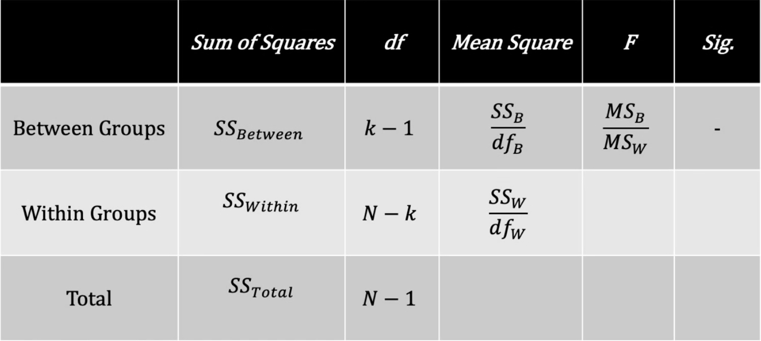
The overall variability in the dataset is called Sum of Squares Total (SS_total). To calculate it the grand mean of the dataset is subtracted from each value, then squared and summed.

The between-conditions variability is denoted as Sum of Squares Between (SS_between). It is calculated by subtracting the grand mean out of the means for each group, and squaring that value, the final value is multiplied by the number of participants in each group. The sum of these values for each group gives us the between-conditions variability.

To calculate the variability within-conditions you subtract the SS_between out of SS_total. Another option is to subtract the group means out of each group’s raw scores, then square and sum the values. The sum of the results will give you the SS_within.

It is important to understand however, that these values are uncalibrated regarding the number of participants. This could be done using Degrees of Freedom:

df_total: N - 1: The entire sample

df_between: k - 1: Group means

df_within: N - k: Entire sample minus number of groups

The calibrated values of variability are called Mean Squares (MS). They are calculated by dividing the SS by its corresponding df. Only after completing this step can we compare the variability and make a decision if most of it is accounted to the between-conditions or within-conditions variability. To do that we divide the MS_B by the MS_W which gives us the F-ratio.

One-Way ANOVA Assumptions:

1. Level of Measurement: has to be interval or ratio

2. Random Sampling

3. Independence of Observations: the observations that make up the data have to be independent of one another - cannot have one participant in multiple conditions (no repeated-measures) - violation dramatically increases likelihood of Type I Error

4. Normal Distribution for each group

5. Homogeneity of Variances can be overlooked if the group sizes are reasonbly similar