[Unit 7, 8, 9] All procedures AP STATS
1 sample Hypothesis Test
Parameter:
“Let µ equal _____”
H0:µ = __ and Ha:µ (</>/≠) __
Conditions:
The problem states the sample was chosen at random
Less than 10% of total population 10(n)< population
n>30, CLT applies. Graph if n<30. “Approximately normal, no outliers”
One sample t-test:
STAT → TEST→ 2 [T-TEST]
Conclusion
if p < α, then the null hypothesis is rejected, indicating that there is sufficient evidence to support the alternative hypothesis.
if p > α, we failed to reject the null hypothesis
2 Sample T-interval for means

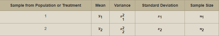
Parameter:
“Let µ1 equal _____ µ2 equal____”
We want to estimate the difference between the mean of ___ and ___ at a α% confidence level
Conditions:
The problem states the samples were chosen at random for each sample
Less than 10% of total population 10(n)< population
n>30, CLT applies. Graph if n<30. “Approximately normal, no outliers”
All 3 conditions for both samples!
2 Sample T interval :
STAT → TEST→ 0 [2-SAMP-T-INT]
State all input and output
Conclusion
"We are % confident the difference of the true population mean of __________ and the true population mean of _________ is between ___ and ____.."
2 Sample Hypothesis Test for means
Parameter:
“Let µ1 equal _____ µ2 equal____”
H0:μ1−μ2=0 or H0:μ1=μ2
Ha:μ1−μ2 >/</≠ 0 or Ha:μ1 >/</≠ μ2
Conditions:
The problem states the samples were chosen at random for each sample
Less than 10% of total population 10(n)< population
n>30, CLT applies. Graph if n<30. “Approximately normal, no outliers”
All 3 conditions for both samples!
2 sample t-test:
STAT → TEST→ 0 [2-SAMP-T-TEST]
State all input and output
Conclusion
if p < α, then the null hypothesis is rejected, indicating that there is sufficient evidence to support the alternative hypothesis.
if p > α, we failed to reject the null hypothesis
Matched Pairs— one-sample t-test
These paired data typically occur in before-and-after situations, when two observations are made of the same individual, or one observation is made of each of two similar individuals.
µd= mean difference
Parameter:
“Let µ equal _____”
Ha:µd=0
Ha:µd>0
Ha:µd<0
Ha:µd≠0
Conditions:
The problem states the sample was chosen at random
Less than 10% of total population 10(n)< population
n>30, CLT applies. Graph if n<30. “Approximately normal, no outliers”
Same sample size, samples are paired
One sample t-test:
STAT → TEST→ 2 [T-TEST]
make sure to input the DIFFERENCE of the 2 samples into L1
Conclusion
if p < α, then the null hypothesis is rejected, indicating that there is sufficient evidence to support the alternative hypothesis.
if p > α, we failed to reject the null hypothesis
Linear regression test
The statistical values found using sample data help estimate population parameters α and β to create μy = α ± βx, where α represents the intercept and β is the slope.
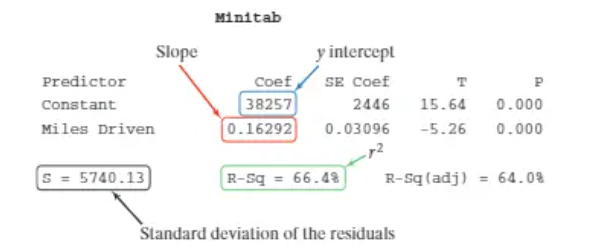
Parameter:
Let β equal the true slope of the regression line for predicting y from x. Most often, you will determine whether the slope of the regression line is equal to zero, making the null hypothesis
H0:β=0.
If the slope of the line is zero, then there is no linear relationship between the x and y variables.
Ha:β≠0, There is a linear relationship
>0, related positively
<0, related negatively
Conditions:
L: Linear— the scatterplot of the data is approximately linear
I: Independent— Must be from a random sample, the values of x and y are independent of each other
N: Create a plot of the RESIDUAL and ensure independence
E: Standard deviation should be the same. The residual plot must have equal scattering both above and below the line
R: Data came from well designed experiment OR randomized experiment
Calculations:
(b-β0)/st deviation = t
tcdf for p value
Conclusion
if p < α, then the null hypothesis is rejected, indicating that there is a linear relationship between ___ and ___
Linear regression Interval
Parameter:
Let β equal the true slope of the regression line for predicting y from x.
We are estimating the true slope of the population regression for predicting y in contest of x.
Conditions:
L: Linear— the scatterplot of the data is approximately linear
I: Independent— Must be from a random sample, the values of x and y are independent of each other
N: Create a plot of the RESIDUAL and ensure independence
E: Standard deviation should be the same. The residual plot must have equal scattering both above and below the line
R: Data came from well designed experiment OR randomized experiment
Calculations:
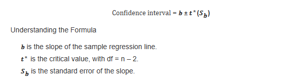
Conclusion
We are __% confident that the slope of the true linear relationship between [the y variable] and [the x variable] is between [lower value] and [upper value].
Chi square [Goodness of Fit]
Parameter:
H0: All the proportions are equal to the claimed population proportions.
“H0:p1=0.25,p2=0.25,p3=0.25,p4=0.25
Ha: At least one of the proportions in H0 is not equal to the claimed population proportion.”
Ha: At least one of the proportions in H0 is not equal to the claimed population proportion.
Conditions:
Simple random sample: The data must come from a random sample or a randomized experiment.
Expected counts: All expected counts are at least five. You must state the expected counts.
chi square goodness of fit test:
stat, test, D (𝛘2GOF–Test)
Hand calculate:
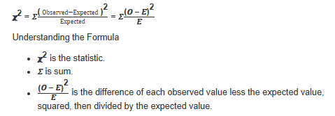
then use chi cdf
df= n-1
Conclusion
We either reject/fail to reject the null hypothesis that all of the proportions are as hypothesized in the null because the p-value is greater than/less than the level of significance. There is/is not sufficient evidence to suggest that at least one of the proportions are not as hypothesized.
if the p is low, the null got to go!
if p < α, then the null hypothesis is rejected, indicating that there is sufficient evidence to support the alternative hypothesis.
if p > α, we failed to reject the null hypothesis
Chi square [test for independence]
Compares the counts from a single group for evidence of an association between two categorical variables
Two-way table
One sample and two categorical variables
Data collected at random from a population and two categorical variables observed for each unit
Parameter:
H0: The row and column variables are independent (or they are not related).
Ha: The row and column variables are not independent (or they are related).
Conditions:
Simple random sample: The data must come from a random sample or a randomized experiment.
Expected counts: All expected counts are at least five. You must state the expected counts.
chi square:
DF= (number of rows-1)(numbers of columns - 1)
Expected values by hand:
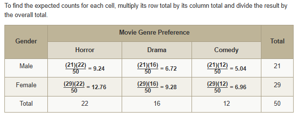
To find it by calc, use Matrices (2nd x^-1). Input the table in matrix a (exclude totals) and leave matrix b blank, then, use the chi square test (STAT → TEST → C)
Conclusion
if the p is low, the null got to go!
if p < α, then the null hypothesis is rejected, indicating that there is sufficient evidence to support the alternative hypothesis.
if p > α, we failed to reject the null hypothesis
There is/is not sufficient evidence to suggest the row and column variables are not independent (or they are related).
Chi square [test for homogeneity]
Compares the distribution of several groups for one categorical variable
Two-way table
Two samples and one categorical variable
Data collected by random sampling from each subgroup separately
Parameter:
H0: The proportions for each category are the same (or p1=p2,p3=p4,p5=p6).
Ha: The proportions for at least one category is different, or not all of the proportions stated in the null hypothesis are true.
Conditions:
Simple random sample: The data must come from a random sample or a randomized experiment.
Expected counts: All expected counts are at least five. You must state the expected counts.
chi square:
DF= (number of rows-1)(numbers of columns - 1)
Expected values by hand:
To find it by calc, use Matrices (2nd x^-1). Input the table in matrix a (exclude totals) and leave matrix b blank, then, use the chi square test (STAT → TEST → C)
Conclusion
if the p is low, the null got to go!
if p < α, then the null hypothesis is rejected, indicating that there is sufficient evidence to support the alternative hypothesis.
if p > α, we failed to reject the null hypothesis