AP Statistics complete guide (includes all tests)
Unit 1
when asked to describe a scatterplot, remember to talk about your DOFS!
Direction: Positive or negative?
Outliers: Are there any apparent outliers?
Form: Linear or nonlinear?
Strength: Strong (points are close to the regression line) or weak (points are further away)?
Residual plots are used to determine if current linear models are appropriate, if it has random scatter, it means that the current model is appropriate, if there is a clear pattern, another model will fit the data better.
TLDR: Random = good, pattern = bad
Residuals = y - y-hat
Actual - Predicted (Think AP statistics!)
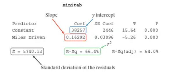
R-squared/Coefficient of determination interpretation: [r-squared percentage] of the variation in [y] can be accounted for by the variation in [x].
Y-intercept interpretation: When [x in context] is zero, the predicted [y in context] is [b units]
Slope interpretation: On average, for each additional increase in [x in context], the predicted [y in context] changes by [slope units]
1 sample Hypothesis Test
Parameter:
“Let µ equal _____”
H0:µ = __ and Ha:µ (</>/≠) __
Conditions:
The problem states the sample was chosen at random
Less than 10% of total population 10(n)< population
n>30, CLT applies. Graph if n<30. “Approximately normal, no outliers”
One sample t-test:
STAT → TEST→ 2 [T-TEST]
Conclusion
if p < α, then the null hypothesis is rejected, indicating that there is sufficient evidence to support the alternative hypothesis.
if p > α, we failed to reject the null hypothesis
2 Sample T-interval for means

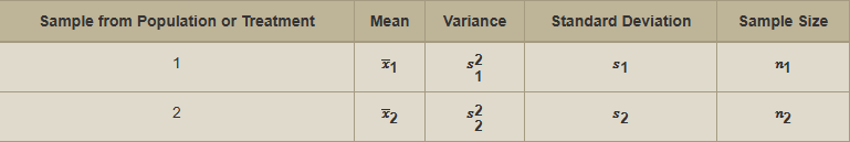
Parameter:
“Let µ1 equal _____ µ2 equal____”
We want to estimate the difference between the mean of ___ and ___ at a α% confidence level
Conditions:
The problem states the samples were chosen at random for each sample
Less than 10% of total population 10(n)< population
n>30, CLT applies. Graph if n<30. “Approximately normal, no outliers”
All 3 conditions for both samples!
2 Sample T interval :
STAT → TEST→ 0 [2-SAMP-T-INT]
State all input and output
Conclusion
"We are % confident the difference of the true population mean of __________ and the true population mean of _________ is between ___ and ____.."
2 Sample Hypothesis Test for means
Parameter:
“Let µ1 equal _____ µ2 equal____”
H0:μ1−μ2=0 or H0:μ1=μ2
Ha:μ1−μ2 >/</≠ 0 or Ha:μ1 >/</≠ μ2
Conditions:
The problem states the samples were chosen at random for each sample
Less than 10% of total population 10(n)< population
n>30, CLT applies. Graph if n<30. “Approximately normal, no outliers”
All 3 conditions for both samples!
2 sample t-test:
STAT → TEST→ 0 [2-SAMP-T-TEST]
State all input and output
Conclusion
if p < α, then the null hypothesis is rejected, indicating that there is sufficient evidence to support the alternative hypothesis.
if p > α, we failed to reject the null hypothesis
Matched Pairs— one-sample t-test
These paired data typically occur in before-and-after situations, when two observations are made of the same individual, or one observation is made of each of two similar individuals.
µd= mean difference
Parameter:
“Let µ equal _____”
Ha:µd=0
Ha:µd>0
Ha:µd<0
Ha:µd≠0
Conditions:
The problem states the sample was chosen at random
Less than 10% of total population 10(n)< population
n>30, CLT applies. Graph if n<30. “Approximately normal, no outliers”
Same sample size, samples are paired
One sample t-test:
STAT → TEST→ 2 [T-TEST]
make sure to input the DIFFERENCE of the 2 samples into L1
Conclusion
if p < α, then the null hypothesis is rejected, indicating that there is sufficient evidence to support the alternative hypothesis.
if p > α, we failed to reject the null hypothesis
Linear regression test
The statistical values found using sample data help estimate population parameters α and β to create μy = α ± βx, where α represents the intercept and β is the slope.
Parameter:
Let β equal the true slope of the regression line for predicting y from x. Most often, you will determine whether the slope of the regression line is equal to zero, making the null hypothesis
H0:β=0.
If the slope of the line is zero, then there is no linear relationship between the x and y variables.
Ha:β≠0, There is a linear relationship
>0, related positively
<0, related negatively
Conditions:
L: Linear— the scatterplot of the data is approximately linear
I: Independent— Must be from a random sample, the values of x and y are independent of each other
N: Create a plot of the RESIDUAL and ensure independence
E: Standard deviation should be the same. The residual plot must have equal scattering both above and below the line
R: Data came from well-designed experiment OR randomized experiment
Calculations:
degrees of freedom: n-2
Conclusion
if p < α, then the null hypothesis is rejected, indicating that there is a linear relationship between ___ and ___
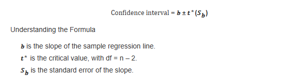
Linear regression Interval
Parameter:
Let β equal the true slope of the regression line for predicting y from x.
We are estimating the true slope of the population regression for predicting y in contest of x.
Conditions:
L: Linear— the scatterplot of the data is approximately linear
I: Independent— Must be from a random sample, the values of x and y are independent of each other
N: Create a plot of the RESIDUAL and ensure independence
E: Standard deviation should be the same. The residual plot must have equal scattering both above and below the line
R: Data came from well designed experiment OR randomized experiment
Calculations:
Conclusion
We are __% confident that the slope of the true linear relationship between [the y variable] and [the x variable] is between [lower value] and [upper value].
Chi square [Goodness of Fit]
Parameter:
H0: All the proportions are equal to the claimed population proportions.
“H0:p1=0.25,p2=0.25,p3=0.25,p4=0.25
Ha: At least one of the proportions in H0 is not equal to the claimed population proportion.”
Ha: At least one of the proportions in H0 is not equal to the claimed population proportion.
Conditions:
Simple random sample: The data must come from a random sample or a randomized experiment.
Expected counts: All expected counts are at least five. You must state the expected counts.
chi square goodness of fit test:
stat, test, D (𝛘2GOF–Test)
Hand calculate:
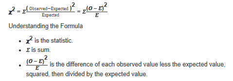
then use chi cdf
df= n-1
Conclusion
We either reject/fail to reject the null hypothesis that all of the proportions are as hypothesized in the null because the p-value is greater than/less than the level of significance. There is/is not sufficient evidence to suggest that at least one of the proportions are not as hypothesized.
if the p is low, the null got to go!
if p < α, then the null hypothesis is rejected, indicating that there is sufficient evidence to support the alternative hypothesis.
if p > α, we failed to reject the null hypothesis
Chi square [test for independence]
Compares the counts from a single group for evidence of an association between two categorical variables
Two-way table
One sample and two categorical variables
Data collected at random from a population and two categorical variables observed for each unit
Parameter:
H0: The row and column variables are independent (or they are not related).
Ha: The row and column variables are not independent (or they are related).
Conditions:
Simple random sample: The data must come from a random sample or a randomized experiment.
Expected counts: All expected counts are at least five. You must state the expected counts.
chi square:
DF= (number of rows-1)(numbers of columns - 1)
Expected values by hand:
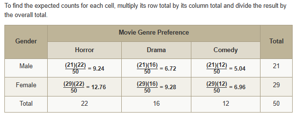
To find it by calc, use Matrices (2nd x^-1). Input the table in matrix a (exclude totals) and leave matrix b blank, then, use the chi square test (STAT → TEST → C)
Conclusion
if the p is low, the null got to go!
if p < α, then the null hypothesis is rejected, indicating that there is sufficient evidence to support the alternative hypothesis.
if p > α, we failed to reject the null hypothesis
There is/is not sufficient evidence to suggest the row and column variables are not independent (or they are related).
Chi square [test for homogeneity]
Compares the distribution of several groups for one categorical variable
Two-way table
Two samples and one categorical variable
Data collected by random sampling from each subgroup separately
Parameter:
H0: The proportions for each category are the same (or p1=p2,p3=p4,p5=p6).
Ha: The proportions for at least one category is different, or not all of the proportions stated in the null hypothesis are true.
Conditions:
Simple random sample: The data must come from a random sample or a randomized experiment.
Expected counts: All expected counts are at least five. You must state the expected counts.
chi square:
DF= (number of rows-1)(numbers of columns - 1)
Expected values by hand:
To find it by calc, use Matrices (2nd x^-1). Input the table in matrix a (exclude totals) and leave matrix b blank, then, use the chi square test (STAT → TEST → C)
Conclusion
if the p is low, the null got to go!
if p < α, then the null hypothesis is rejected, indicating that there is sufficient evidence to support the alternative hypothesis.
if p > α, we failed to reject the null hypothesis