FW 453: Stage Structured Growth, 2/11-2/18

FW 453: Stage Structured Growth, 2/11-2/18

Review

• Our pop growth models have been

  • limited to a single term (lambda or r)

  • applied to an entire pop

• Today, we transition to acknowledging individuals of different (st)ages have different contributions to pop growth

Stage Vs Age

Stages can depend on actual age, but also developmental, morphological, or potentially behavioral stages.

Stage structured growth

• We can answer questions like

• does shooting adult cormorants have the same effect on pop growth as oiling their eggs?

• how many female deer need to be sterilized to reduce their abundance? is that the same as effect as harvesting adult males? juveniles harvested?

• what management options would be most efficient at recovering endangered bighorn sheep? protect adults or increase connectivity for juveniles?

• what are the effects of different stressors on sage grouse pop growth? are these effects uniform across stage classes and sex?

Sea turtles

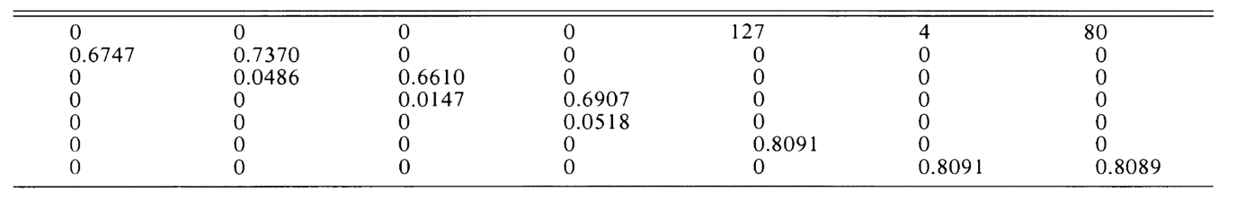
To create a stage-based projection matrix, we must estimate, for each stage, the reproductive output (Fi), the probability of surviving and growing into the next stage (G,). and the probability of surviving and remaining in the same stage (P,). The fecundities Fi are given in Table 3. The transition probabilities Gi and Pi can be estimated from the stage- specific survival probabilities pi and stage duration di

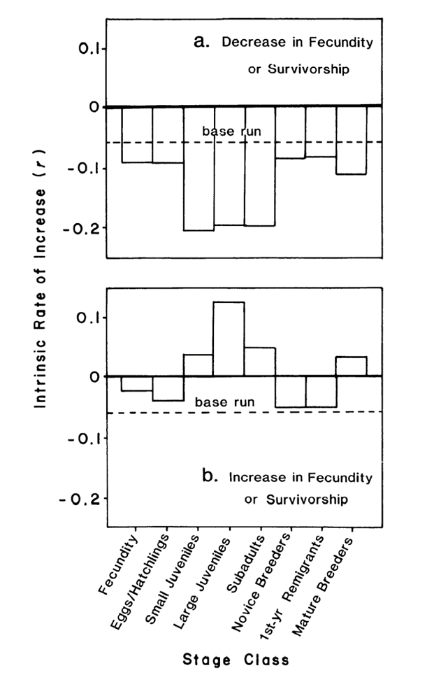
• Eggs, hatchlings

• Small juveniles

• Large juveniles

• Subadults

• Novice breeders

• 1st-yr remigrants

• Mature breeders

• 50% decrease in survival or fecundity

• 50% increase in fecundity or an increase in survivorship to 1.0 (100% survival)

• using population analysis to manage species

  • even if hatchling survival were increased to 100%, loggerheads would decline

  • instead, pop growth rate was most responsive to decreasing mortality of juveniles and secondarily mature adults

  • because of these, Turtle Excluder Devices (TEDs) were required to be installed in shrimp nets

  • the number of turtles killed in nets declined by about 44% after TED regulations were implemented

  • has helped increased turtle recovery

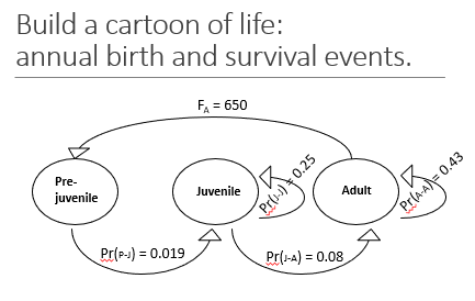
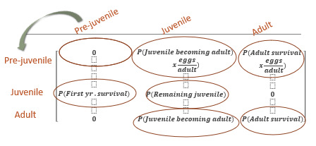
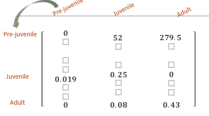
Example: Common frogs

• frog species found throughout europe

• vital rates and abundance for

  • pre juveniles (egg, tadpole, overwintering metamorph form)

  • juveniles (considered juvenile for 2 years)

  • adults (may live multiple years)

• how to project abundance T years into the future

Structure to numbers

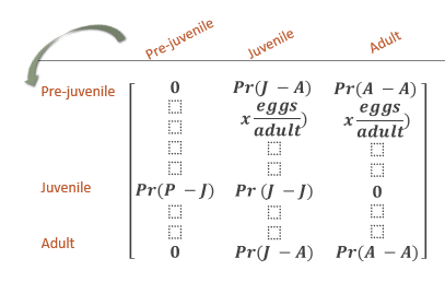
• A population-projection matrix is just an organized way to project a population forward one time step

• 

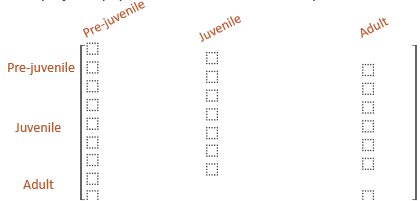
• The "population projection matrix" describes the number of offspring born to each stage class that survive a given time period as well as the proportion of individuals in each stage class that survive and remain in that stage

  • vs. those that survive and enter another stage, otherwise known as the "transition probability."

• Thus the elements of the matrix A incorporate the fecundity, mortality, and growth rates of each stage class.

• The Leslie matrix divided the population into equal age classes.

• In the Lefkovitch matrix, there is no necessary relation between stage and age; the fundamental assumption is that all individuals in a given stage are subject to identical mortality, growth, and fecundity schedules.

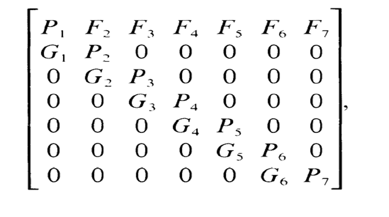
Matrix review

• The top row of the matrix is not just number of offspring (fecundity)

  • rather it refers to reproductive contribution to the next time step (number of offspring x survival)

• The diagonals are the probabilities of surviving and remaining in the same stage class

• The sub-diagonals are the probabilities of surviving and transitioning to the next stage class

Matrix example

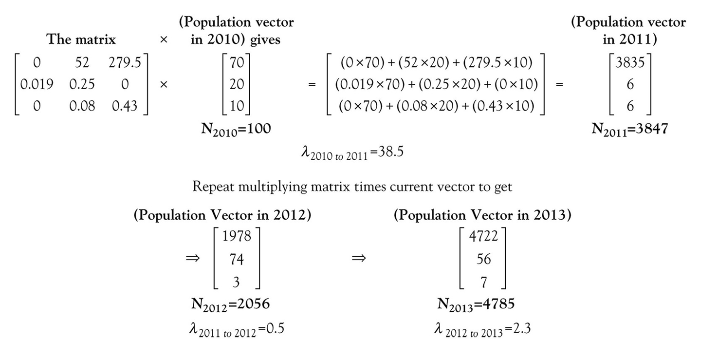
n(t+1) = M*n(t) (6.1)

M_r x c (rows by columns)

3 rows and 1 column, so 3 by 1 pop vector for [ 70 20 10 ] (vertical down)

M_3×3 x N_3×1 = A_3×1 (multiply by outer components)

Basically, multiply each number in a row in a matrix by the numbers in the pop vector. So, if we had [0, 52, 279.5] and a pop vector of [70 20 10] (vertical down), it would be [(0×070) + (52×20) + (279.5 × 10)] and so forth going down the original matrix multiplying the numbers.

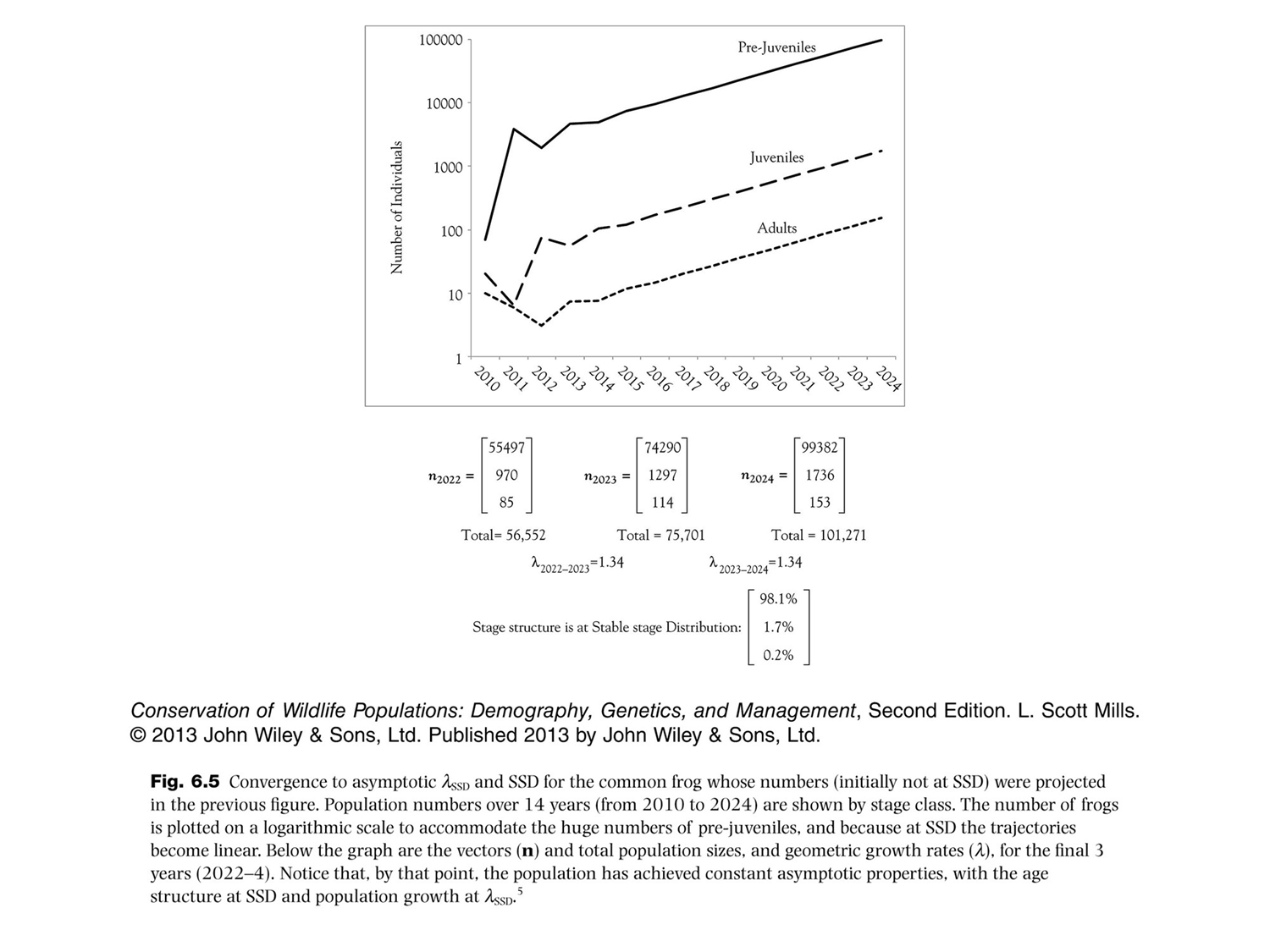
Stable Stage Distribution (SSD)

• Under relatively constant conditions, any stage structured pop will converge on a constant pop growth rate

  • This constant growth rate is called “asymptotic lambda” (will also appear as lambda_SSD)

• Another result is a “stable stage distribution” (SSD)

  • this just means the proportion of individuals in each (st)age class will become constant over time

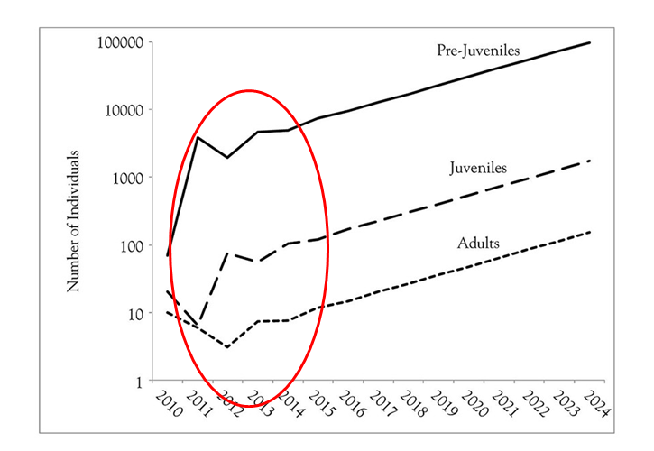
• The amount of time it takes to reach SSD and asymptotic lambda can depend on a number of factors

  • initial stage distribution—how different initial conditions are from SSD

  • generation time

  • overall, usually occurs within 20 time steps

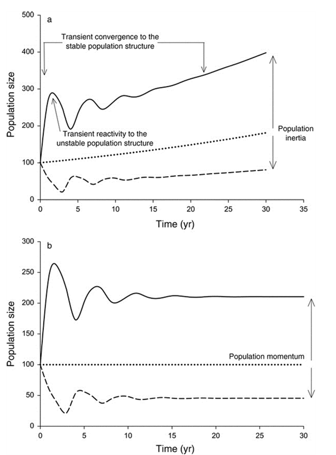
• This progression from crazy fluctuations to SSD is called “transient dynamics”

  • probably very common in real world

    • harvest

    • translocations

  • 

Class Mantras

• all vital rates are NOT CREATED EQUAL

• all ages or stages are NOT CREATED EQUAL

• all management actions are NOT CREATED EQUAL

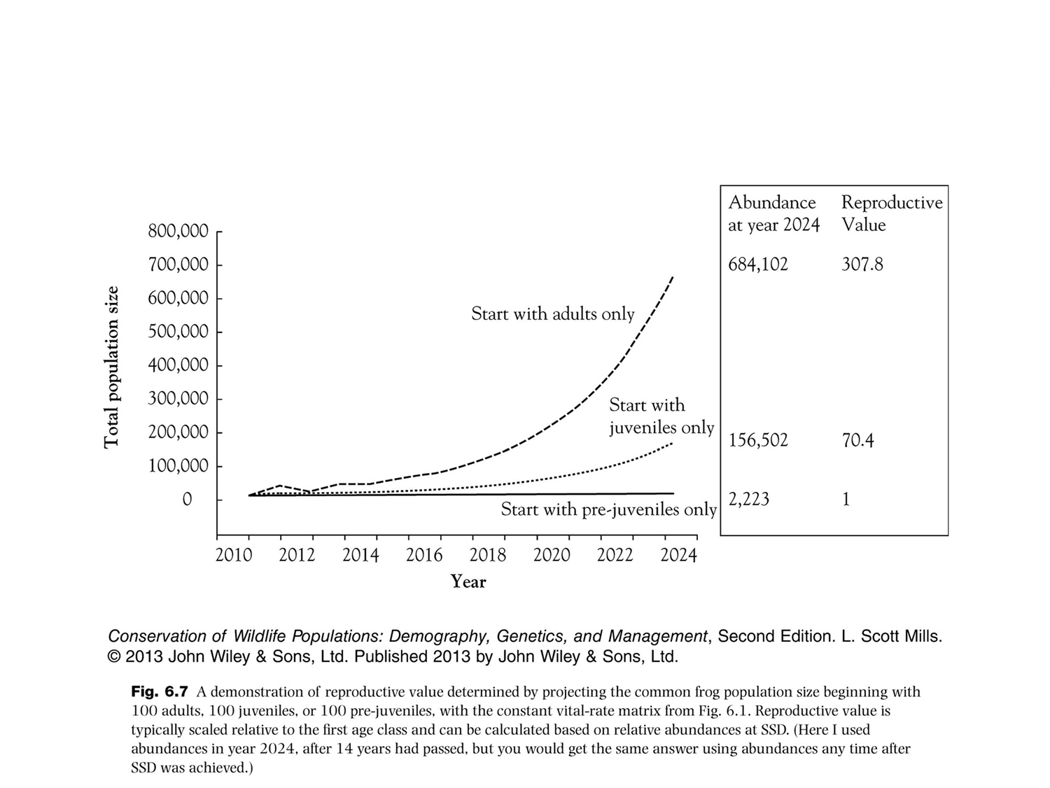
The key to understanding transient dynamics: Reproductive Value

• “Reproductive value” captures the relative ‘importance’ of each stage to future pop growth

• another way to describe RV is “a measure of the force each stage class has on future pop growth”

  • it is the weighed average of present and future reproduction, accounting for pop growth rate

• Reproductive Value (RV) depends on current and future reproduction, which depends on survival. it also depends on pop growth rate

• think about applied potential for this concept

• not the same as “reproduction”!!

• reproductive value can be determined using matrix math or it can be determined… how?

Reproductive Value

• Common frog example—seeding method

  • three pops of 100 frogs

    • same vital rates (projection matrix)

    • each pop only has one stage class (e.g. 100 pre juveniles, 0 juveniles, 0 adults)

  • Would each of these pops have the same number of frogs over time?

  • Why?

    • remember the mantras!

      • all stage classes are not created equal

        • they have very different RVs

• Depending on the relative overabundance vs. underabundance of particular phenotypic classes (e.g., adults vs. offspring), the initial transient reaction to an unstable population structure can lead to sudden and substantial increases or decreases in population size

• In addition to the particular instability of population structure, an organism’s generation time will influence the rate at which stable population structure is achieved and the magnitude of transient fluctuations in abundance en route to the stable dynamics.

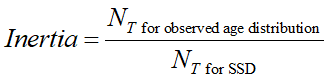
• These unstable short-term dynamics can in turn produce an inertial effect on long-term population size causing it to be larger or smaller than that of an otherwise equivalent population that always has a stable population structure, which we call ‘‘population inertia’’

Recap

• All stages are not equal in the effects on pop grwoth

  • each stage has different reproductive value and stable stage distributions

  • initial conditions (i.e. initial stage distributions) greatly affect

    • transient dynmaics (magnitude and time length)

      • no stochastic forces are present—simply a result of deviation of initial distribution from SSD

    • initial pop growth

    • future pop size

    • time required to reach SSD

• How do you determine SSD of any pop?

• how do you determine RV of different stage classes?

Review

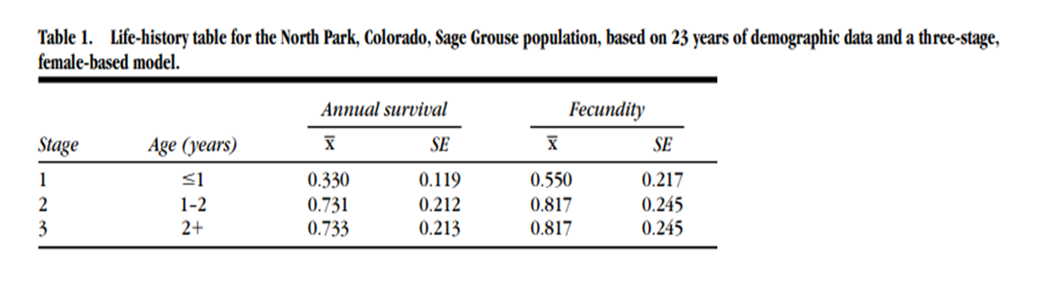
• Scenario: Greater sage grouse are in notable decline across most of their range due mostly to landscape fragmentation (oil and gas development), overgrazing by cattle on public lands (vegetation degradation), and antiquated sagebrush removal programs (habitat loss). Twenty-three years of demographic data in the North Park Valley of Colorado found the following information:

• Task 1: Create a ‘cartoon of life’ for sage grouse with vital rates appropriately labeled

• Task 2: Translate cartoon of life into population projection matrix

• Task 3: Project population forward one time step and calculate lambda

• Starting N: Stage 1 = 38, Stage 2 = 14, Stage 3 = 38

• 

Sensitivity Analysis

Sensitivity Analysis Answers:

• Which model entry (i.e. vital rate) has the greatest influence on population growth rate (λ)??

• …And directs management!

• Sea turtle story

  • 50% decrease in survival or fecundity

  • 100% survival or 200% fecundity

  • 

Analytical sensitivities and elasticities

• “importance” of individuals in different stages arises from the fact that all vital rates are NOT created equal

• So, in management we have to consider both

  • how much a change in that vital rate affects pop growth AND

  • how much we can change each vital rate

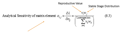
• What determines the importance of different vital rates to pop growth?*

  • reproductive value (call it v_i)

  • what proportion of pop is that stage class (SSD: call it w_i)

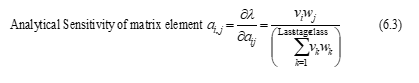
• Determining how much a tiny change in stage-specific vital rates affect growth rate: “Analytical Sensitivity”

  • how sensitive pop growth is to changes in different vital rates

  • (understand biology, don’t memorize)

  • 

  • think about what this is, biologically. based on that, what is a way you could calculate sensitivities in excel without using calculus or derivatives? (will work for either matrix element or component)

  • Elasticity is just the scaled (proportional) sensitivity

• So “analytical sensitivity” (and elasticity) tell us some general rules for which tiny changes in vital rates affect pop growth the most, but what is missing for us rough-and-tumble, real-world applied biology types?

  • 

    • Tells us nothing about what happens when changes are big

    • tells us nothing about when multiple changes happen at once

    • do you want to live life making infintesimal, one at a time changes?

We need to think about how to incorporate…

• Variation in vital rates AND

• management-releveant changes

Real World Variation Can be Incorporated into Matrix Models

• Demographic stochasticity

  • constant mean vital rates lead to variable # surviving and being born, just due to sampling whole animals

• Environmental stochasticity

  • good years, bad years

  • mean vital rates change each year

  • also complications like correlations among rates and over time

And you can learn about how to actually incorporate stochasticity and what affects it has on stage-structured pops

• in the section p 109 through p 113

  • stochasticity in age and stage-structured populations

• we’ll consider that to be optional reading that you are not required to do

Now let’s talk about how to save the world by helping to design more efficient wildlife management actions through sensitivity analysis

Sensitivity Analysis

• three approaches

  • manual changes

  • analytical sensitvity and elasticity analysis

  • life-stage simulation analysis (lsa) “simulation based sensitivity analysis”

Manual perturbations (changes)

• manually change the input of a pop model

  • can be big or small

  • able to explroe predicted outcomes of management options

    • change vital rate by some specified, expected amount (or range of values)

  • not limited to investigating importance of vital rates—explore biologically relevant factors and the effect of different age structures

Analytical sensitivity and elasticity analysis

• we already did this!

• measure how different vital rates affect pop growth if changed by very small and equal amounts

  • say nothing about how vital rates actually change in nature or under management! (variability in a vital rate)

Can build uncertainty into sensitivity analysis with a “life-stage simulation analysis”

Know what this is but don’t need to know how to do it.

1. create thousands of what if scenarios

2. Draw vital rates from distributions derived from field data

3. simulate 100s of pop matrices from the vital rates

4. summarize growth rate, vital rates, SSD from the simulated matrices

5. regress lambda values from matrices against each vital rate to look at how much of the variation in growth rate is explained by variation in that vital rate (largest R²)

Case Study: Red cockaded woodpeckers (RCW)

RCW management actions determined from a clever matrix model

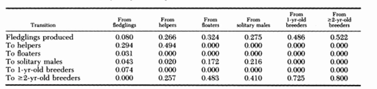
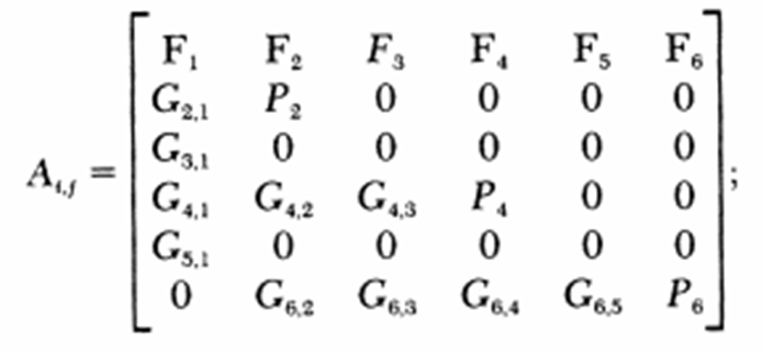
• used management relevant manual perturbations

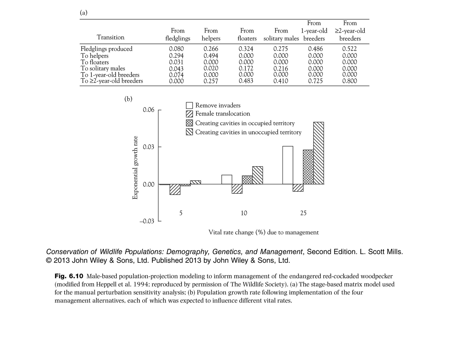
Management Actions

1. Remove invaders: remove cavity invaders such as flying squirrels and other woodpecker species that inhabit red-cockaded woodpecker nest cavities, increasing woodpecker fecundity.

2. Female translocation: capture and relocate female red-cockaded woodpecker fledglings to solitary male territories, causing more solitary males to become breeders.

3. Cavities in occupied territories: drill cavities in existing territories, increasing the fecundity of breeders and the probability that fledglings become helpers while decreasing the chance that fledglings become breeders.

4. Cavities in unoccupied territories: increase new territories by drilling artificial cavities in unused yet suitable habitat and by reducing hardwood understory. This action should increase both fledgling-to-breeder and helper-to-breeder transitions while decreasing fledgling mortality.

Used manual perturbations combined with elasticity analysis…

Case Study: Brown-headed cowbird

• How to best control cowbirds?

  • remove eggs?

  • remove adults?

  • other action?

• Elasticity of nestling, and yearling survival is equal, but more variation in egg survival thus greatest effect on lambda

• look at R² to find that the egg survival rate explains the most variation