Unit 1: Limits and Continuity
1.1 Intro to limits
A limit is one of the most fundamental concepts of calculus. The limit of a function at is the numerical value approaches as we get closer and closer to .
We can write limits in limit notation as , which is pronounced “the limit of as approaches .
Graphed to the right is the function . As an example, lets approximate .
Recall that is the numerical value that approaches as gets closer and closer to . Examining the graph, we can see that .
However, it might also be tempting to say that because . This is a common fallacy many students make when evaluating limits—we must always remember that .
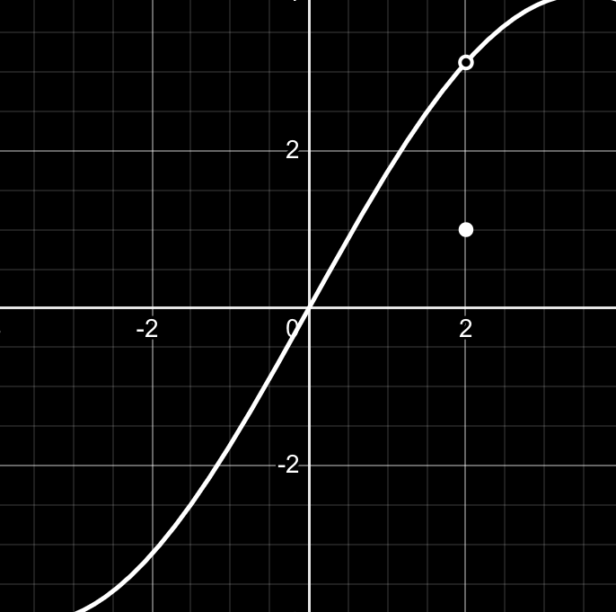
When we evaluate limits, we want to think about what happens as gets infinitely close. What this means is that we can always get as close to the limit as we want.
For example, if we want to find a limit , we want to think about and so on. We also want to think about and so on.
Lastly, for a limit to exist, it must approach the same value from both sides. If a limit approaches a different value from the left of than from the right of , then we can say that does not exist.
1.2 Estimating limits from graphs
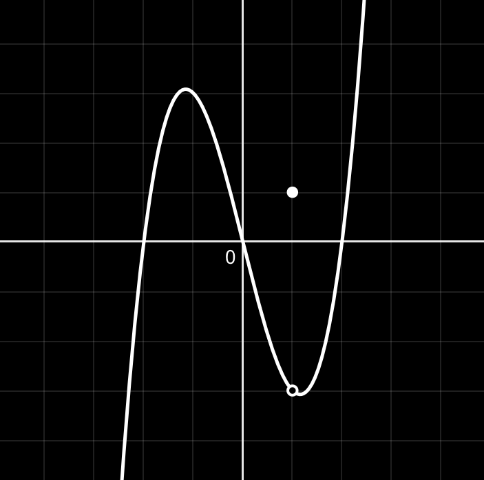
Earlier, we introduced the idea that . Let’s reinforce this idea by examining two graphs. In both examples, we will attempt to find the limit .
Example 1
To approximate , we need to determine what the -values around are approaching as we get closer and closer to .
Although , , because as approaches , approaches .
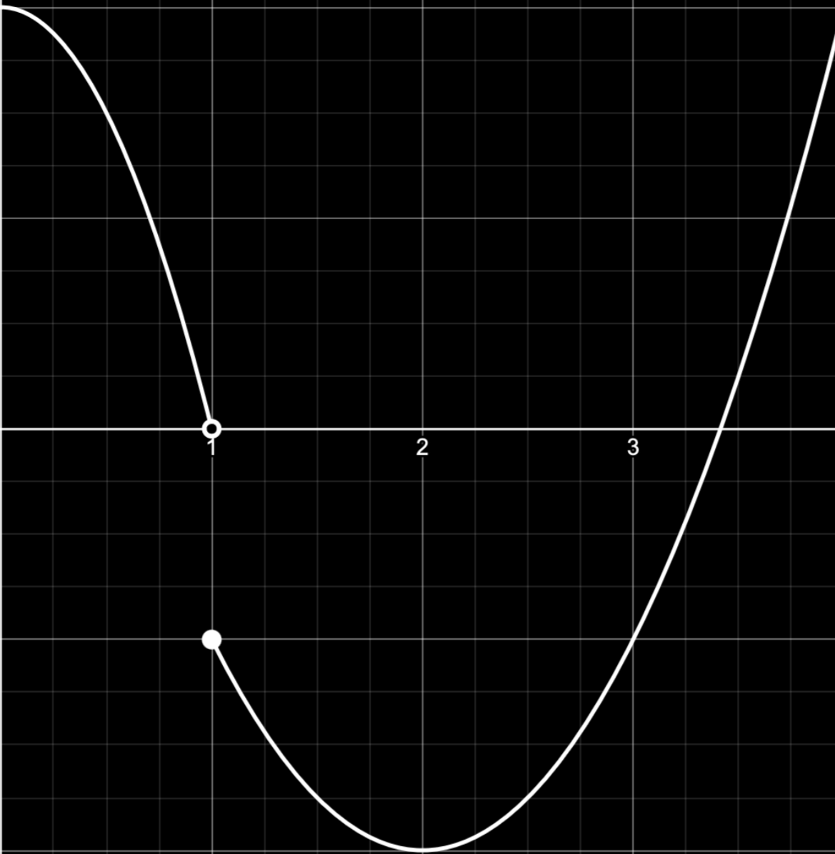
Example 2
To approximate , we need to determine what the -values around are approaching as we get closer and closer to .
Although , is undefined because as approaches , approaches from -values less than and from values greater than .
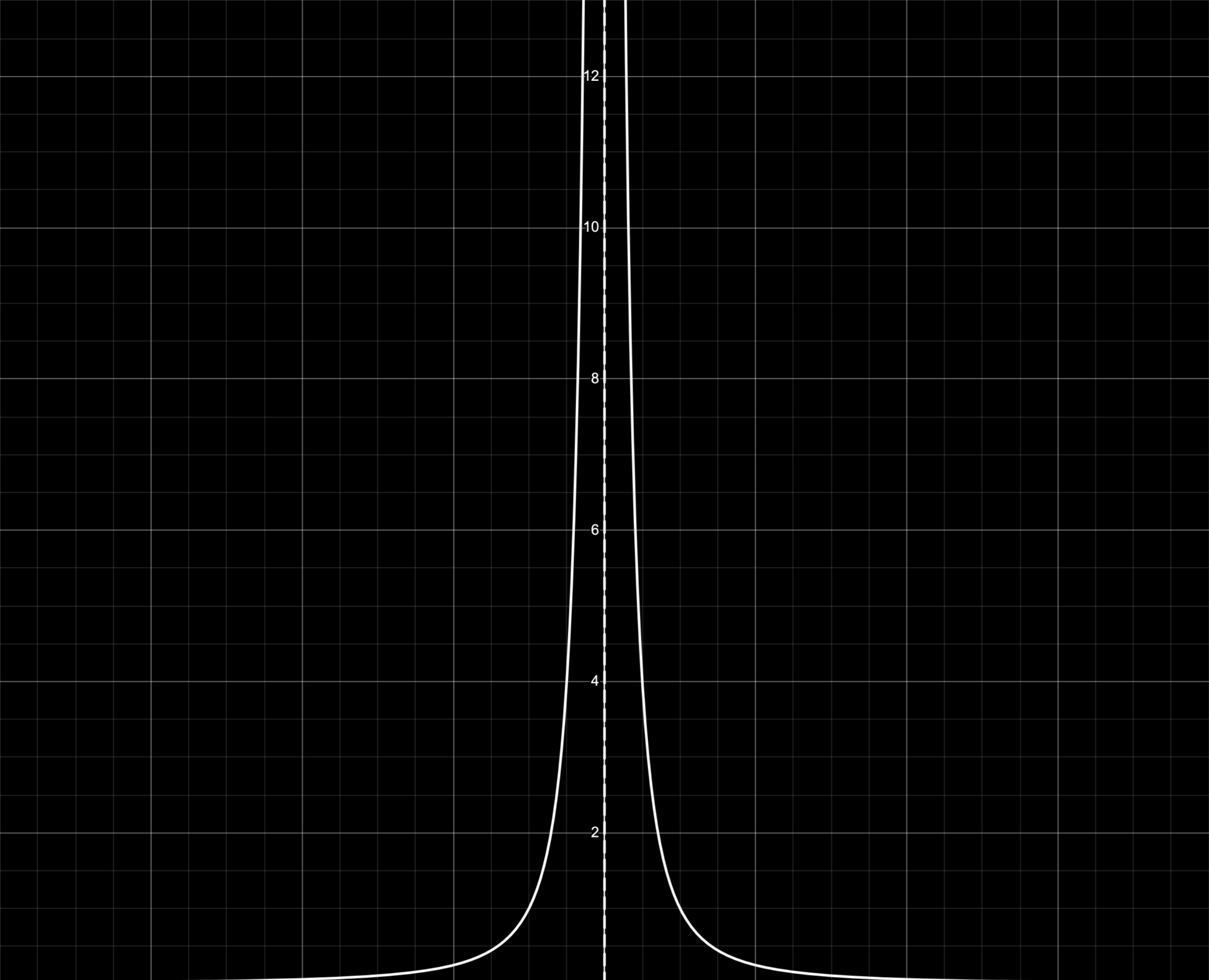
An unbounded limit occurs when we attempt to take the limit of a vertical asymptote. At a vertical asymptote, the function we try to take the limit of skyrockets to infinity without ever touching the -value it is at. So, when we try to approximate what a function approaches at a vertical asymptote, we will find that the limit does not exist because the function never approaches anything.
We can see an unbounded limit in the example above when we try to take the limit . The function never approaches anything, so does not exist.
Earlier, we introduced the idea that if a limit approaches two different values from both sides, it is undefined. We can rewrite this idea by saying that a limit is undefined if its two one-sided limits are different. Lets discuss what a one-sided limit is:
A positive one-sided limit describes a limit from values that are greater than , or from the right of . We denote positive one-sided limits with a superscript “+” sign in the limit notation, as .
On the flip side, a negative one-sided limit describes a limit from values that are less than , or from the left of . We denote negative one-sided limits with a superscript “-” sign in the limit notation, as .
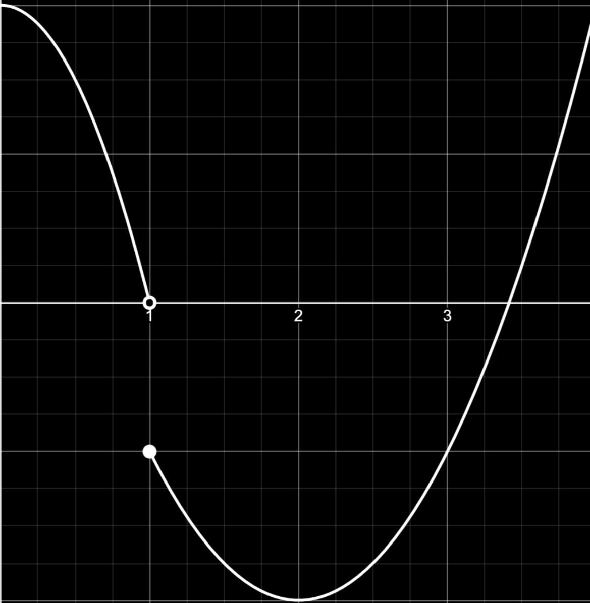
Looking at our example (which is shown to the left for convenience) from above, lets try to find the one-sided limits at .
When we approach from the left, approaches . So, .
When we approach from the right, approaches . So, .
What we said above can now be written as “ is undefined if .”
1.3 Estimating limits from tables
Before we begin estimating limits from tables, we need to be able to accurately create appropriate tables for approximating limits. There are a few things that we need to make sure we consider, listed below:
We need to simulate getting infinitely close to the limit by selecting values that approach the limit from both sides. As an example/reminder, if we want to evaluate a limit , we want to consider and so on. We also want to consider and so on.
This also means not approaching the limit in constant increments. We want to decrease the distance to the point of interest, not keep it the same.
We also want to make sure that we approach the limit from both sides. This means that we need to consider