Stats chapter 4& 5

Basics
Nomenclature:
The variables we use to predict are called the explanatory variables or predictors. They are denoted as X
The variables that are predicted are called response or outcome variables. It is denoted as Y.
Identify the variables:
1. Suppose a study is conducted to predict the daughter’s height based on the mother’s height.
2. Suppose the local fishing community wishes to predict the age of fish based on their scales.
3. Suppose we wish to predict the mileage of a car based on its engine size.
Visualization: The primary tool for examining the relationship between 2 numerical variables is a scatter plot.
We will now plot the home price data. What do we look for in a scatter plot?
• Trend
• Strength
• Shape
Example 1:

What is Trend?
The general tendency of the scatter plot as you read from left to right.
1) Increasing (uphill) – positive association
2) Decreasing (downhill) – negative association
3) No trend – mass of points with no clear pattern
What is Strength?
Recall we discussed the wider horizontal spread with respect to histograms, dot plots
having higher standard deviation and vice versa. Here in a scatter plot, we look for vertical
spread.
a) Scatter plots with large amounts of scatter or vertical variation indicate a weak
association.
b) Scatter plots with small amounts of scatter or vertical variation indicate a strong
association.
What is shape?
The simplest shape is linear, and we apply the methods we learn here only to linear shapes
When describing a scatter plot, we should include the following:
a) Trend
b) Strength
c) Shape
Note: Always use the phrase “tends to” when describing an association. Always point out any data
points that appear to be unusual or not part of the general pattern.
4.2: Correlation Coefficient
Given a scatterplot, we can find its trend, strength, and shape. Can we quantify the strength of the
variables?
The correlation coefficient is a number that measures the strength and direction of the linear
relationship between the two numerical variables X and Y. It is denoted by the symbol r and -1 ≤ r ≤ 1.
If r = -1, then there is a strong negative linear relationship.
If r = 1, then there is a strong positive linear relationship.
If r = 0, then there is no association.
Simple linear regression
Let us do a scatter plot, compute r and interpret it for the following data: (heights and weights of 6 women)

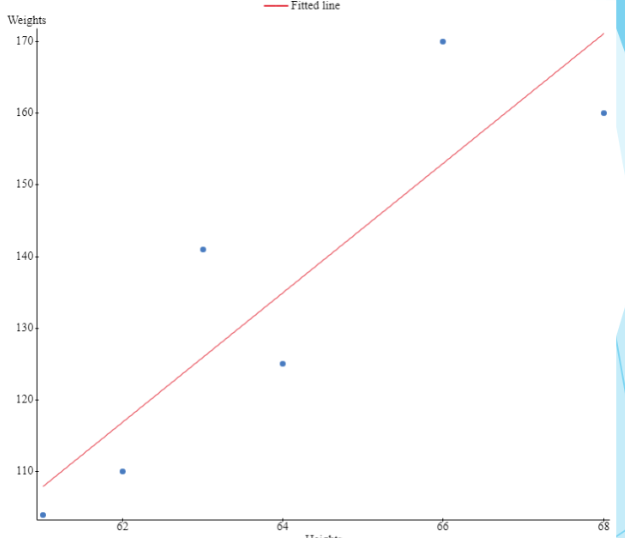
Simple linear regression results:
Dependent Variable: Weights
Independent Variable: Heights
Weights = -442.88235 + 9.0294118 Heights
Sample size: 6
R (correlation coefficient) = 0.88093363
R-sq = 0.77604407
(Do this using a calculator)
SLR continued:
a) Changing the order of the variables does not affect r. (redo the previous example with
X = Weights, Y = Heights)
b) Adding a constant or multiplying by a positive constant does not affect r.
c) r is unitless.
d) r makes sense only if the relationship is linear.
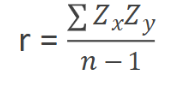
Formula for R :
Regression line: A tool for predicting future observed values. It also provides us
with a useful way of summarizing a linear relationship between two numerical variables.
Recall from algebra, y = mx + c
In Linear Regression, we write the regression line as follows: (explain using the scatter plot)
䒠 䔠 䕠 䕀ℎ 䘐 䘀= -442.88235 + 9.0294118 Heights
Response variable = Weights
Predictor = Heights
Slope = 9.0294118
Y-intercept = -442.88235
Slope Interpretation: For every unit increase in height, there is an increase of 9.029 units of weight on
average.
Y-intercept Interpretation: The weight of a woman with height = 0 inches is -442.88 lbs. (Most of the
time, the y-intercept does not make any sense).
Definitions
Outliers: The correlation coefficient and the regression line are both sensitive to outliers.
Influential points: An influential point is a point that changes the regression equation by a large amount. Not all outliers are
influential points.
Extrapolation: Making predictions beyond the data range. Never do this. Only interpolation is possible.
Coefficient of determination: This is simply the square of the correlation coefficient. We usually multiply it by 100 to get the
percentage.
If r² = 100 %, then we have a perfect linear relationship, and the regression line perfectly predicts the responses.
If r² = 0%, then there is no linear relationship, and the regression line does not predict well.
Advantage of r²: It measures how much variation in y (response) is explained by x (predictor).
Lurking variable: It is a variable which is not included in the study either as an explanatory
or a response variable but can affect the interpretation of the relationship between variables.
It is like a confounding variable in observational studies.
Eg: Ice cream sales and long lines at the beach are correlated. The lurking variable here is
_____________.
Note: Association, not causation!!!